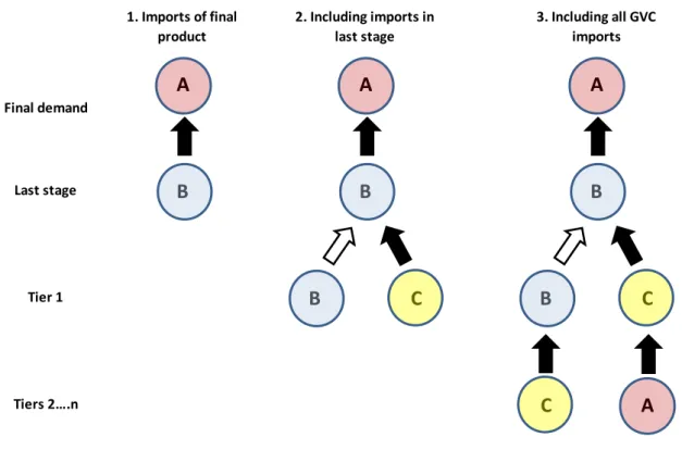
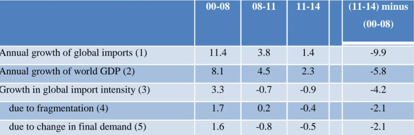
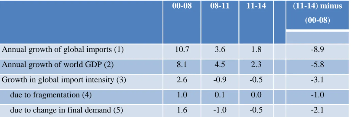
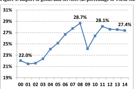
We denote the relationship between GVC imports and the value of the final product by the term 'global import intensity' of production. Note: The import intensity of production (per gross output unit) is based on first-stage imports only and including all imports in the GVC as defined in equation (9).
16 Keeping the values in A at period 0 levels, we can write
Data from updated World Input-Output Database (WIOD)
For this article, we developed an update of the World Input-Output Database (WIOD). WIOT and WIOD are built within the framework of the latest system of national accounts and take into account its concepts and accounting identities.
Results
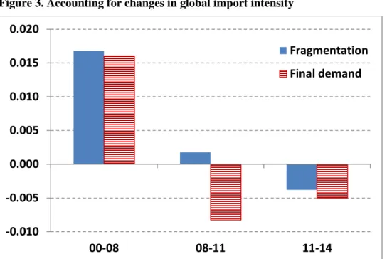
- Accounting for the import intensity of global final demand
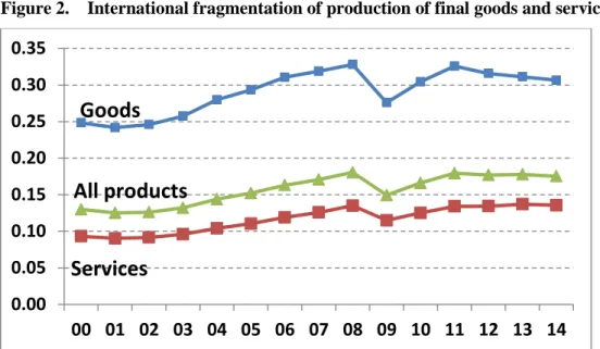
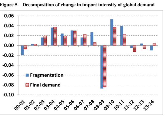
- Trends in international production fragmentation
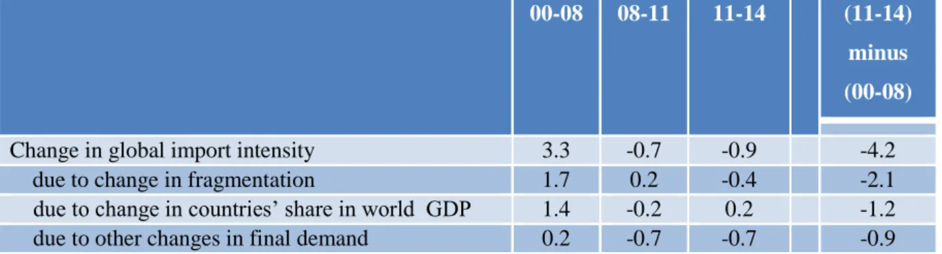
Broken down into the contribution of the change in GVC imports and the change in the structure of global final demand, see Table 2. We present new evidence on the global import intensities (GII) of the production of 2,464 final goods and services in the world economy. For example, we provide GII related to the production of final motor vehicles ("cars").
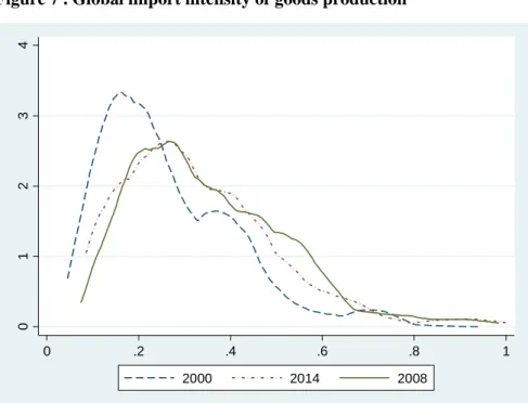
In Figure 7 we provide a kernel density plot of GIIs for the 836 commodity GVCs for which we have data, namely final output from 19 manufacturing industries in 44 finalization countries. Densities are presented for the years 2014 and 2014, and observations are weighted with nominal final output values. The total sample consists of 11,889 observations, which are weighted by the final output value of the value chain.30 Figure 8 shows the estimated coefficients for the year models and the associated 95 percent confidence intervals.
For the first time, we are also able to analyze international fragmentation in the production of services.
27 4.3 Global import intensity of countries’ final demand
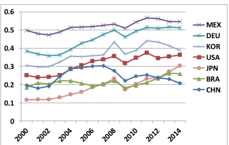
Contribution to change in global import intensity through change in the share of countries in global final demand. Country contributions are calculated according to equations (23) using country-specific import intensities relative to the world average. China's share of global demand is growing rapidly, but the import intensity of its final demand is well below the world average.
As shown in Figure 11, GII of Chinese final demand was briefly above the world average in the early 2000s, but has since trended downward. This is because Chinese final demand is increasingly shifting to services, but also because it requires fewer imports as more and more products are produced locally. European countries typically have high import intensities, but the decline in global demand was not large enough to have a significant impact on the slowdown in import intensity at the global level.
32 It should be remembered that we analyze the import intensity of final domestic demand, which excludes imports for exports.
30 5. Concluding remarks
As a final comment: We do not claim that this exercise provides a causal analysis of the drivers of global trade. Our findings on international production fragmentation highlight the importance of including endogenous evolution of global supply chain structures in such models. 2016), The Great Convergence: Information Technology and the New Globalization, Harvard University Press. Why is world trade so weak and what can policy do about it?”, OECD Economic Policy Papers no. ed.), The Global Trade Slowdown: A New Normal?, A VoxEU eBook, London: CEPR Press and EUI.
Understanding the Weakness in Global Trade: What is the New Normal?”, ECB Occasional Paper Series Noguera (2012), “Accounting for Intermediates: Production Sharing and Value Added Trade”, Journal of International Economics. An Illustrated User Guide to the World Input-Output Database: Case of Global Automotive Production.”, Review of International Economics.
Natural resources are defined as products produced by the Mining Industry (WIOD industry 4) and the Petroleum Refining (industry 10).
36 Appendices
WIOD 2016 is an update of WIOD 2013, which contains the same type of data and tables and is produced using the same methodology. Compared to the previous version, the new WIOD includes three more countries: Norway, Switzerland and Croatia. The new version of WIOD is structured according to recent industry and product classification viz.
However, it should be noted that – due to the new SNA methodology and (sometimes large) revisions to the National Accounts series and the lack of one-to-one correspondence between the old and new industry classifications – they cannot be linked just together. The commodity dimension is according to the CPA2008 classification and covers 56 commodities corresponding to the main products of the 56 industries listed in Appendix Table A1. In general, the construction of WIOD 2016 follows the same methodology as the 2013 release, as described extensively in Timmer et al. 2015) and in more technical detail in Dietzenbacher et al.
Two improvements have been made, making better use of data that have become available in recent years.
38 Bilateral trade shares
Therefore, we had to compromise in the construction of the WIOT, and decided to focus on the construction of a basic price version as the most desirable. In the construction of the WIOT from the international SUTs, a final adjustment had to be made, to transform the bilateral exports back from fob to a basic price basis. Note that this is a reasonable assumption as it concerns the margins in the exporting country.
In WIOT this is final consumption expenditure by households (CONS_h) plus final consumption expenditure by non-profit organizations serving households (CONS_np). 𝐼 is Investment, or gross capital formation: in WIOT this is gross fixed capital formation (GFCF) plus changes in inventories and valuables (INVEN). For these columns, the values in all adjustment rows for the columns in WIOT (taxes less subsidies on products, Cif/fob adjustments on exports, Direct purchases abroad by residents, Domestic purchases by non-residents) are included.
Net tax on exports is not given in the VOET, but can be found in the International SUT for the country.
47 Austria
48 Croatia
49 Estonia
50 Greece
51 Italy
SNA08 tables at basic prices are available from EUROSTAT for the years 2010-2012 External time series. SNA08 tables at basic prices are available from EUROSTAT for 2010 External time series. The 2012 shares of detailed A64 industries in their A21 sector aggregate are used to apportion unallocated 2013 A64-level industry output.
Therefore, quarterly GDP data at the A10 level were used to extrapolate the value-added series up to 2014. The 2013 gross output-value-added ratios are used to estimate the 2014 industry-level gross output data A64. SNA08 purchase price application tables and basic offer price tables are available for 2010 and 2011 from EUROSTAT.
Value added growth rates at the national level are used to estimate missing values.
54 Slovak Republic
We left the total values in the rows and columns for H52 since there are no shares available to do the split. We also assume that all product output is produced in-house, so that GRAS could be used to estimate the missing cells. In the use table, the supply table GO shares are used to estimate the industry totals to allocate the unallocated total intermediate use by industry.
For the product totals, the same was done using the distribution of total supply at basic prices to allocate the unallocated total intermediate use by product from which the interior of the use table was estimated. There is no 2008 SNA93 Use or IO table at basic prices for the UK. The values for the cells were retrieved using information from row and column totals that were available and applying GRAS technique.
Therefore, the 2013 gross output to value added ratios were used to estimate gross output by industry for 2014.
56 B2 Sources and methods for non-EU Member States
57 External time-series
To obtain further industry detail, the series are split using shares from the input-output tables. Domestic purchases by non-residents and foreign purchases by residents are not reported separately in the national accounts. These are taken from the article "travel" in the balance of payments as published in the China Statistical Yearbooks (accessed April 2016, see link).
Time series of value added and gross output from India KLEMS for the period 2000 to 2011 (available at link). The series are updated using NA statistics on gross output and value added by CSO-detailed industries for the period 2011 to 2013 and broad sectors from 2013 to 2014 (Accessed April 2016 at mospi.nic.in; access requires registration). Input-output tables for and 2010 with producer prices from the national statistics office, Badan Pusat Statistik (BPS).
No information on net taxes is available, so the estimated time series is SUTs at producer prices.
59 External time-series
Dated to 2000 using SUT time series input file based on WIOT, released October 2012. To estimate missing values by industry column in the Use tables for each year, we use GO shares by industry from the supply table in the year relevant. To estimate missing values by product row in the EUROSTAT usage tables for 2010 and 2011, we use the product distribution for total supply from the supply table.
For 2014, output data at the industry level A64 is not fully completed, but EUROSTAT A21 sector level totals are available. The 2013 shares of detailed A64 industries in their A21 sector aggregate are used to distribute unallocated output to A64-level industries for 2014. User warning: due to the scarcity and outdated nature of publicly available Russian statistical data, we do not advise users to use this data to make analysis of the Russian economy.
We included Russia in this version of the WIOD only for analyzes of international trade with Russia.
61 SUTs
62 SUTs
63 Turkey
The totals for Intermediate Use (II) by producing industry are derived as the difference between GO and VA for each industry. We distribute the Row NA totals of II and FD by manufacturing industry using the total distribution of the WIOD countries Brazil, India, China, Indonesia, and Mexico. This gives an initial IO matrix of II and FD by producing industry for which GO by producing industry is not necessarily the same as GO by using industry.
From international SUTs, it is known for RoW for each manufacturing industry how much it exports to WIOD countries and in which industries the products are used. At this stage, imports are included in the RoW IO matrix, so IMP by manufacturing industry is added to GO by manufacturing industry. It is known from international SUTs how much RoW is imported from WIOD countries by manufacturing industry, but not whether it is used for II or FD.
Finally, we subtract the total of Ry inputs by manufacturing industries from the Ry IO table to obtain the domestic Ry blocks for II and FD.