Accepted Manuscript

We show that the intensity of product competition (i.e., the degree of product differentiation) and consumer switching behavior play important roles in determining equilibrium sampling strategy. When product competition is strong and no consumer switching behavior occurs, competitive retailers always adopt symmetric sampling strategies. However, if consumer switching behavior exists and/or product competition is relatively weak, retailers may begin to adopt asymmetric sampling strategies.

How are the retailers' sampling and pricing strategies affected by the intensity of product competition, consumer switching behavior and the goodwill effect of sampling. Our finding shows that when the intensity of competition is strong (i.e., a low degree of horizontal product differentiation such as substitute products), and no consumer switching behavior occurs, competing retailers reach symmetric equilibria—. When the intensity of product competition becomes relatively weak, the retailers can also reach asymmetric equilibria even without consumer switching behavior.

Therefore, consumer switching behavior and the intensity of product competition play an important role in determining the equilibrium sampling strategy. Some existing literature suggests that consumer switching behavior intensifies price competition (Klemperer 1987a, 1987b and Farrell and Klemperer 2007). In contrast to the simultaneous-move game, we find that in a sequential game, competitive retailers can adopt asymmetric sampling strategies even if the intensity of competition is strong and there is no consumer switching behavior.

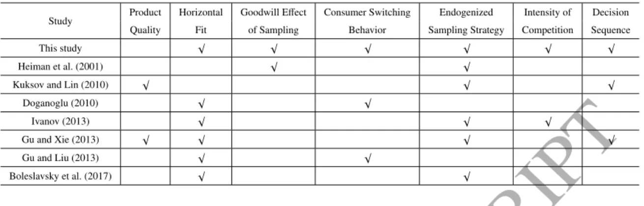
In contrast, this paper illustrates how the competitive firms' strategy of revealing adaptation is affected by consumer switching behavior, the goodwill effect of sampling, and the intensity of product competition.

Table 1: Research on Information Revelation Strategy

ACCEPTED MANUSCRIPT

Equilibrium Sampling Strategy under Simultaneous Decisions

For the No Sample-Sample strategy, consumers can only resolve fit uncertainty for one product and therefore cannot tell the extent of differentiation between the two products. Therefore, the extent of horizontal product differentiation (ie, the intensity of competition) does not affect the profits of the two retailers. Second, in the No Sample-Sample strategy, the information disposition of the sampled retailer establishes the spread of consumers' posterior valuations across products, thereby creating a perceived differentiation among the retailers' products.

Specifically, in the No Sample–Sample strategy, consumers can realize their ex post evaluations of the sampled seller, but their ex ante evaluations of the unsampled one remain. When both retailers offer free samples (i.e., the sample-sample strategy), consumers maintain the same ex ante V¯ + ∆V valuation of both products before traveling to the retailers. The intensity of competition (ie, the degree of horizontal product differentiation) begins to affect the profits of the two retailers.

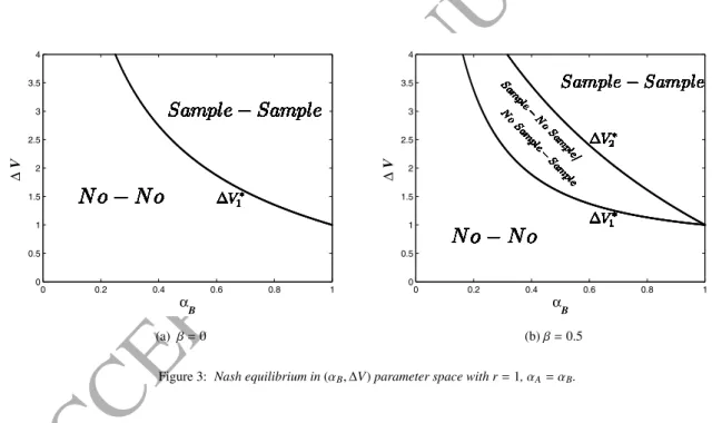
These mechanisms explain why the Nash equilibrium is a sample-sample equilibrium when the probability of realizing a good fit is high and the goodwill effect of sampling is strong, as shown in Figures 3a and 3b. In Figure 3b, with the switching behavior of the consumer, the non-sample–sample/sample–no-sample Nash equilibrium exists in the range ∆V ∈ [∆V1∗,∆V2∗]. Furthermore, as shown in Figure 3, ∆V1∗and ∆V2∗ decrease as αB increases in [0,1] (ie, sample-sample Nash equilibrium usually exists for large αB).

Interestingly, when the intensity of product competition is strong, both retailers can make more profit under the No–No strategy than under the Sample–Sample strategy. When the intensity of competition is high, that is, the degree of product differentiation is low, competing traders find themselves in a prisoner's dilemma when they reach the Sample–Sample Nash equilibrium. We also find that, in the case of intermediate intensity of competition, competing retailers may not fall into a prisoner's dilemma when they reach sample–sample equilibrium if there is consumer switching behavior.

This result differs from that in the case of a strong competitive intensity, where retailers enter the captive dilemma when they reach the sample-sample equilibrium (see Theorem 6). Consumer switching behavior can therefore benefit both retailers in the sample-sample equilibrium and cause this equilibrium to become dominant. Therefore, when ∆V becomes large, the Nash equilibrium shifts from No–No to Sample–No Sample (or No Sample–Sample) and then to Sample–Sample.

Note that the sample-sample equilibrium in Figure 5b covers a larger area than that in Figure 5a. That's because when the intensity of competition is weak, consumer switching behavior benefits both retailers in the sample. When the intensity of competition is weak, i.e. the degree of product differentiation is high, retailers are more likely to achieve the Sample-Sample Nash equilibrium with a greater consumer switching rate.

Figure 3: Nash equilibrium in (α B , ∆V ) parameter space with r = 1, α A = α B .

Equilibrium Sampling Strategy under Sequential Decisions

When competitive intensity is weak, competing retailers may employ asymmetric sampling strategies even if no consumer switching behavior occurs (i.e., β = 0), as shown in the left and right regions of Figure 5a. Moreover, in cases with a weak intensity of competition, a Sample–. Sample strategy can dominate a no-no strategy for competing retailers and there can be no prisoner's dilemma. To solve the Stackelberg game, we first find follower B's optimal sampling and pricing strategies for any given pricing and sampling decision by leader A. Based on the follower's sampling and pricing responses, we solve for the leader's optimal sampling and pricing strategies.

This phenomenon occurs in the No–No and Sample–Sample scenarios with high competitive intensity. But in a sequential game, one of the retailers – the follower – can observe the price strategy of the leader and follow it. With such a response from the follower, the leader would charge a higher price and encourage the follower to charge a higher price as well.

In a sequential move game, when the intensity of product competition is strong, the equilibrium sampling strategy is as follows. In the case where all consumers have high switching costs (ie β= 0), the equilibrium is a trial-trial equilibrium if∆V >∆V21sst∗; it is a sample-no sample equilibrium if∆V ∈[∆V11sst∗,∆V22sst∗]; otherwise it is a No-No equilibrium. In particular, ∆V11sst∗ is the threshold at which it makes no difference to the manager to adopt a Sample–No Sample strategy or to adopt a No–No-Sample strategy; ∆V12sst∗ is the threshold at which the manager's profit in a Sample–Sample strategy is the same as in a No Sample–Sample strategy;∆V13sst∗ is the threshold at which the manager obtains the same profit in a Sample–No Sample strategy as in a No Sample–Sample strategy; ∆V21sst∗ is the threshold at which it makes no difference to the follower to provide sampling or no sampling since the leader applies no sampling.

V22sst∗ is the threshold at which it makes no difference for the follower to provide sampling or no sampling, given the leader providing sampling. Similar to the results in a simultaneous game, retailers are more likely to reach the sample-to-sample equilibrium when the goodwill effect of sampling is strong, and they tend to reach asymmetric equilibria when the probability of a good match to be realized in a middle interval. Interestingly, Figure 6a and Proposition 9 show that when the intensity of competition is strong, retailers can reach an asymmetric equilibrium (i.e., Sampling–No Sampling) even without consumer switching behavior (i.e., β=0).

The difference occurs because in this Stackelberg game the follower has an advantage over the other player, specifically, the follower can undercut the price of the leader and earn higher profits. In the presence of second-mover advantage, the leader has more and the follower less incentive to exploit the goodwill effect of sampling to attract consumers to visit its store first. In the sequential game, when competing retailers reach asymmetric equilibria, the leader is more likely to adopt sampling while the follower is not to adopt any sampling, as shown in Figure 6 that the region where equilibrium exists is sample–no sample , greater than that a Non-sample–sample equilibrium.

Figure 6: Nash equilibrium in [α B ,∆V] parameter space with r = 1, α A = α B in a Stackelberg Game.

CONCLUSION

If ∆V ≤∆V2∗, Retailer A (B) always chooses no sampling regardless of Retailer B (A's) choice, resulting in competing retailers reaching the No-No Nash equilibrium. If ∆V2∗<∆V<∆V1∗, Retailer A chooses No Sampling as soon as Retailer B chooses No Sampling, and the same decision rule applies to Retailer B, giving competing retailers either the No-No or achieve the No-No. Monster-Monster Balance. It is easy to show that the No-No equilibrium always dominates the Monster-Monster equilibrium in the case with r = 1.

Therefore, they would reach the No-No Nash equilibrium in the region of ∆V2∗ <∆V <∆V1∗. If ∆V ≥∆V1∗, Retailer A (B) always chooses sampling, regardless of Retailer B (A's) choice, causing competing retailers in this region to reach the Sample-Sample Nash equilibrium. If ∆V≤∆V1∗, retailer A (B) always chooses no sampling, regardless of retailer B (A's) choice, resulting in competing retailers reaching the No-No Nash equilibrium.

V ≥∆V1∗, retailer A (B) always chooses sample regardless of the choice of retailer B (A), so competitive retailers reach the Sample-Sample Nash equilibrium in this region. Based on the analysis given in the proof of Proposition 5, we find that in the case withr=1, if∆V1∗≥∆V2∗, retailers never reach the No sampling–sampling or sampling–no sampling equilibrium. They can reach the No sample–sample or sample–no sample equilibrium only if∆V1∗<∆V2∗.

With β=0.5, the region where the Sample–No Sample Nash equilibrium exists overlaps with the region where the No Sample–Sample Nash equilibrium exists. In this overlapping region, it makes no difference whether competing sellers reach the Sample–No Sample or No Sample–Sample Nash equilibrium. By calculation, when β = 0, the No–No equilibrium dominates the Sample–Sample equilibrium; and the opposite is true when β is large.

Furthermore, the Nash equilibrium is the Sample-Sample equilibrium in the region of∆V ≥∆V11wk∗&∆V ≥ ∆V12wk∗. V12wk∗and∆V≥∆V21wk∗&∆V≥∆V22wk∗where the Sample-Sample Nash equilibrium exists expand with a large β. For the above two reasons, retailers are more likely to reach the Sample-Sample Nash equilibrium with a larger β.

Our following result would show that, for the Sample–Sample strategy with a strong competitive intensity, both retailers may be better off in the sequential game than in the simultaneous game. Based on the illustration in the proof of Proposition 9, we show that with β=0, an asymmetric equilibrium, i.e., the Sample–No Sample equilibrium can exist in the region of∆V∈[∆V11sst∗,∆V22sst∗].