A brief history of the finite element method is included, as well as some examples illustrating the application of the method. The introduction of heat transfer exposes the student to additional applications of the finite element method that are most likely new to the student.
Hutton Pullman, WA
I include the appendix only so that the reader is aware of the algorithms underlying the software he/she will use in solving finite element problems. Appendix Includes problems for various chapters of the text to be solved by commercial finite element software.
Basic Concepts of the Finite Element Method
- INTRODUCTION
- HOW DOES THE FINITE ELEMENT METHOD WORK?
- Comparison of Finite Element and Exact Solutions The process of representing a physical domain with finite elements is referred to
- Comparison of Finite Element and Finite Difference Methods
- A GENERAL PROCEDURE FOR FINITE ELEMENT ANALYSIS
- Preprocessing
- Solution
- Postprocessing
- BRIEF HISTORY OF THE FINITE ELEMENT METHOD
- EXAMPLES OF FINITE ELEMENT ANALYSIS
- OBJECTIVES OF THE TEXT
A node is a specific point in the finite element at which the value of the field variable must be explicitly calculated. An excellent history of the finite element method and detailed bibliography is given by Noor [16].

Given the availability of very powerful and sophisticated finite element software packages, why study the theory. As previously mentioned, critical analysis of the results of a finite element model calculation is essential, as those results can ultimately become the basis for design.
Stiffness Matrices, Spring and Bar Elements
INTRODUCTION
The first theorem is the opposite of Castigliano's second theorem, which is more often encountered in the study of the elementary strength of materials [3]. Here, Castigliano's first theorem is used for the specific purpose of introducing the concept of minimum potential energy without resorting to the higher mathematical principles of calculus of variations, which is beyond the mathematical level intended for this text.
LINEAR SPRING AS A FINITE ELEMENT
However, this inverse matrix does not exist since the determinant of the element stiffness matrix is identically zero. Therefore, the constraint does not affect the values of the active displacements (we use the term active to refer to displacements that are unknown and need to be calculated).
ELASTIC BAR, SPAR/LINK/TRUSS ELEMENT
Denoting axial displacement at any position along the length of the rod as u(x), we define nodes 1 and 2 on each side as shown and set the nodal displacements u1 =u(x =0) and u2 =u( x = L) ). Calculate the displacement of the end of the bar (a) by modeling the bar as a single element with a cross-sectional area equal to the area of the actual bar at its midpoint along the length, (b) by two bar elements of using equal length. and similarly evaluate the area at the midpoint of each, and (c) use integration to obtain the exact solution.

STRAIN ENERGY, CASTIGLIANO’S FIRST THEOREM
Formulating the elastic stress energy in terms of the angle of rotation atx=Land shows that Castigliano's first theorem gives the correct expression for the applied torque. For linear elastic systems, the formulation of the stress energy function in terms of displacements is relatively simple.

MINIMUM POTENTIAL ENERGY
The total potential energy includes the stored elastic potential energy (strain energy) as well as the potential energy of the applied loads. Therefore, the total potential energy is expressed as and it can be seen that it is identical to the previous result.
SUMMARY
If we form the matrix triple product 1. 2.58) and perform the matrix operations, we find that the expression is identical to the strain energy of the system. As will be shown, the matrix triple product of Equation 2.58 represents the strain energy of any elastic system.
PROBLEMS
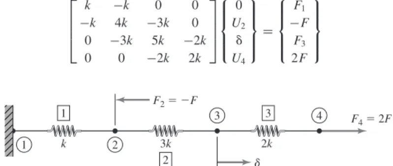
Determine (a) the required values of the forces F2 and F4, (b) the displacement of node 2, and (c) the reaction force at node 1. What other concerns should be considered. 2.11 Figure P2.11 shows an assembly of two rod elements made of different materials.
Truss Structures
The Direct Stiffness Method
INTRODUCTION
The physical properties (in this case, the stiffness matrix and the element strength) of each element must be transformed, mathematically, in the global coordinate system to represent the structural properties in the global system in a stable mathematical frame of reference. In the alternative procedure, known as the flexibility method [1], the displacements are taken as known quantities and the problem is formulated in such a way that the forces (in general, the stress components) are the unknown variables.
NODAL EQUILIBRIUM EQUATIONS
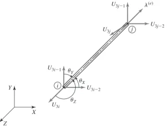
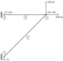
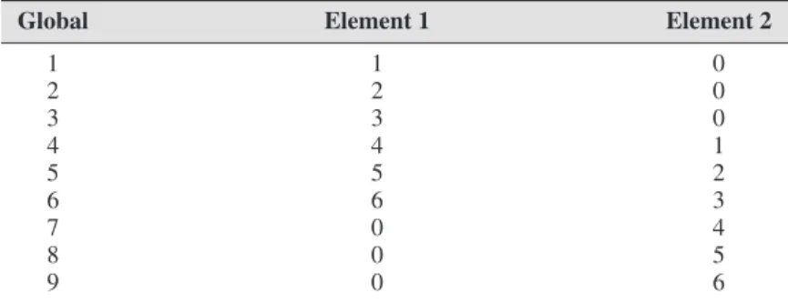
Now to relate element nodal displacements referring to the element coordinates to element displacements in global coordinates, Figure 3.4c shows element nodal displacements in the global system using the notation. U(e)1 = element node 1 displacement in the global X direction U(e)2 = element node 1 displacement in the global Y direction U(e)3 = element node 2 displacement in the global X direction U( e)4 = element node 2 displacement in the global Y direction. b) General displacements of a bar element.
ELEMENT TRANSFORMATION
- Direction Cosines
Comparing this result with Equation 3.18, it is seen that the element stiffness matrix in the global coordinate frame is given by Examination of Equation 3.28 shows that the symmetry of the element stiffness matrix is preserved in the transformation to global coordinates.
DIRECT ASSEMBLY OF GLOBAL STIFFNESS MATRIX
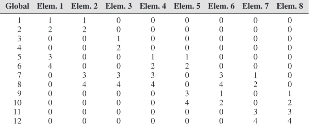
For real calculations, the inclusion of the global displacement numbers within the element stiffness matrix is difficult. Finally, the element stiffness matrix terms are added to the global stiffness matrix using the element displacement location vector.
BOUNDARY CONDITIONS, CONSTRAINT FORCES
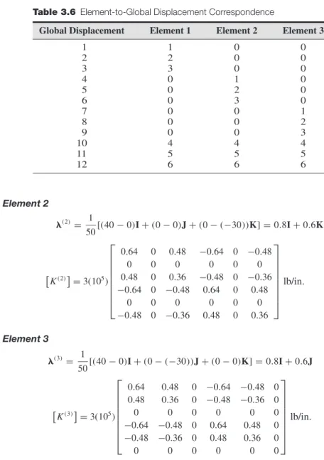
Specification of the cross-sectional area and modulus of elasticity E for each element allows calculation of the element stiffness matrix in the global frame using Equation 3.28. According to the location vector (addresses) of the element, the individual values of the element stiffness matrix are placed in the appropriate mailbox.
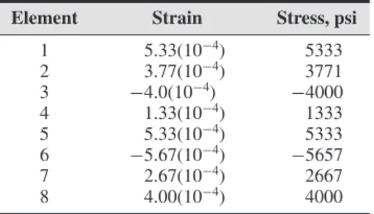
ELEMENT STRAIN AND STRESS
就整体位移而言,杆单元的单元应力由下式给出。
COMPREHENSIVE EXAMPLE
For the present example, the equations are solved using a spreadsheet program, inverting the (relatively small) global stiffness matrix to obtain . The main computational task completed in step 7 provides the displacement components of each node in the global coordinate system.
THREE-DIMENSIONAL TRUSSES
Following the identical procedure used for the 2D case in Section 3.3, the element stiffness matrix in the element coordinate system is transformed to the 3D global coordinates via . Therefore, we only need to compose part of the system stiffness matrix to solve for the three unknown displacements.
SUMMARY
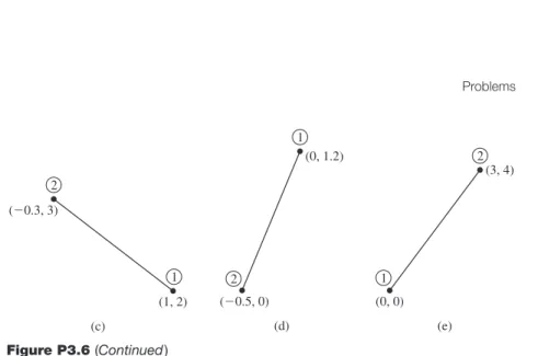
Using the direct stiffness method, determine the deflection of node 2 in the specified global coordinate system and the axial stress in each member. Fit the global stiffness matrix of the system and calculate the global displacements of the unrestricted node.
Flexure Elements
INTRODUCTION
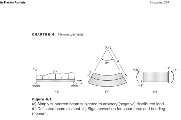
ELEMENTARY BEAM THEORY
Thus we obtain the well-known result that the neutral surface is perpendicular to the bending plane and passes through the center of gravity of the cross-sectional area. Correspondingly, the internal bending moment at a cross-section must correspond to the resultant moment of the normal stress distribution, i.e.
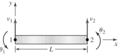
FLEXURE ELEMENT
Substituting Equations 4.22-4.25 into Equation 4.17 and collecting the coefficients of the nodal variables results in the expression Ymax also represents the largest distances (one positive, one negative) from the neutral surface to the exterior surfaces of the element.
FLEXURE ELEMENT STIFFNESS MATRIX
Observing that Equation 4.32 indicates a linear variation of normal stress along the length of the element and since, once the displacement solution is obtained, the node values are known constants, we need only calculate the stress values at the cross-sections corresponding to the nodes; that is, at x = 0 and x = L. For the strain energy of the finite element being developed, we substitute the discretized displacement relation of equation 4.27 to obtain.
ELEMENT LOAD VECTOR
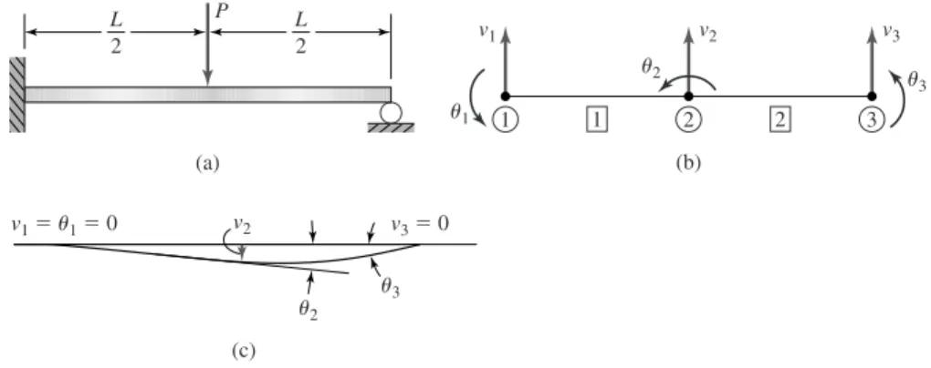
In general, the finite element method is an approximate method, but in the case of the bending element, the results are accurate in certain cases. In this example, the neutral surface deflection equation is a cubic equation and, since the interpolation functions are cubic, the results are exact.
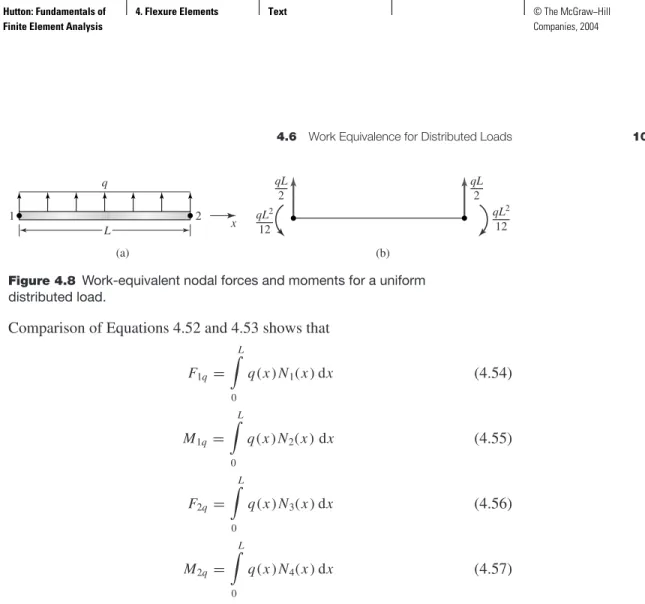
WORK EQUIVALENCE
Collecting the global stiffness matrix for the displacement correspondence table (noting that we use a "short cut" for element 3, since the stiffness of the element in the global X direction is meaningless), we get the results in Table 4.5. We need to examine the numerical behavior of the derived variables after the finite element "mesh" is refined.
FLEXURE ELEMENT WITH AXIAL LOADING
For such applications, the orientation of the element in the global coordinate system must be taken into account, as was the case with the spar element in the beams. Using Figure 4.13, the element displacements are written in terms of global displacements as a) Nodal displacements in the coordinate system of the elements.
A GENERAL THREE-DIMENSIONAL BEAM ELEMENT
The yand axes are assumed to correspond to the principal axes for surface moments of inertia of the cross section[1]. L (x2−x1) =kT(x2−x1) (4.72) Comparison of Equation 4.72 with Equation 2.2 for a linear elastic spring and consideration of the equilibrium state Mx1+Mx2=0 leads directly to the element equilibrium equations:.
CLOSING REMARKS
Using the given stiffness matrix with E=10(106), calculate the deflection of node 2 for the conical element loaded as shown in Fig. P4.18a. Approximate the tapered beam using two planar elements as shown in Fig. P4.18b and calculate the deflection.
INTRODUCTION
METHOD OF WEIGHTED RESIDUALS
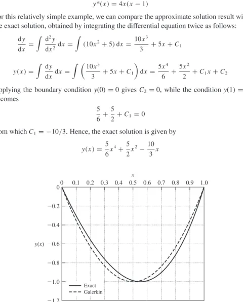
Use Galerkin's method of weighted residuals to obtain an approximate solution of the differential equation. Use Galerkin's method of weighted residuals to obtain a one-term approximation of the solution of the differential equation.
THE GALERKIN FINITE ELEMENT METHOD
- Element Formulation
In light of Equation 5.11 and Figure 5.4b, we see that in any interval xj ≤ x≤ xj+1 only two of the trial functions are non-zero. The interpolation functions correspond to the overlapping parts of the proof functions that apply in a single-element domain.
APPLICATION OF GALERKIN’S METHOD TO STRUCTURAL ELEMENTS
- Spar Element
- Beam Element
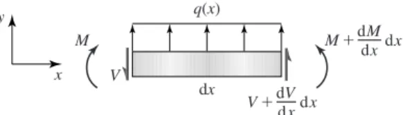
If q(x)=q=constant (positive upwards), substitution of the interpolation functions in equation 5.51 yields the knot force vector element as. If a concentrated force is applied to the node, the sum of the boundary shear forces for the adjacent elements must be equal to the applied force.
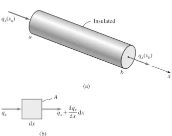
ONE-DIMENSIONAL HEAT CONDUCTION
If no external force or moment is applied to a node, the shear and moment values from Equation 5.52 for adjacent elements are equal and opposite and cancel out in the assembly step. Next, Galerkin's finite element method is applied to Equation 5.59 to obtain the finite element equations.
CLOSING REMARKS
Why the trial function assumed in Example 5.3 does not satisfy the physics of the problem. 5.5(a)–(e) For each of the differential equations given in Problem 5.4, use the method of Example 5.4 to determine trial functions for the binomial approximate solution using Galerkin's method of weighted residuals.
Interpolation Functions for General Element
INTRODUCTION
COMPATIBILITY AND COMPLETENESS REQUIREMENTS
- Compatibility
- Completeness
For a general field problem where the field variable of interest is expressed on an element basis in the discretized form. In the limit, as the element size shrinks to zero in mesh refinement, the field variable and its partial derivatives up to and including the highest order derivative appearing in the integral formulation must be able to assume constant values.
POLYNOMIAL FORMS
Again, due to the discretization, the completeness requirement is directly applicable to the interpolation functions. In addition to consideration of the rigid body motion, the completeness requirement also ensures the possibility of constant values of (at least) the first derivative.
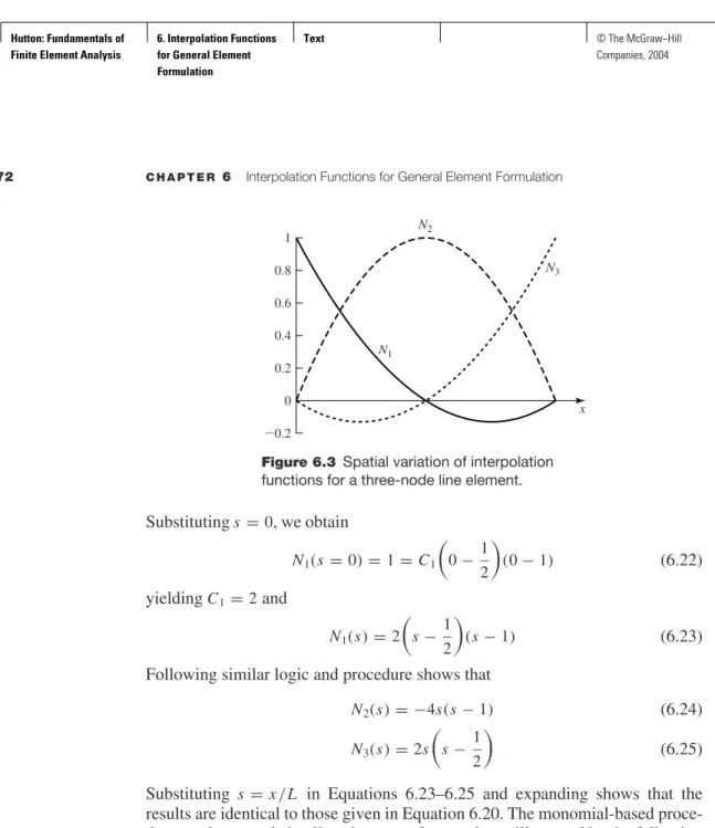
ONE-DIMENSIONAL ELEMENTS
Higher-Order One-Dimensional Elements
These observations lead to an abbreviated method of devising the interpolation functions for a C0 line element as products of monomes as follows. Use the monomial method to obtain the interpolation functions for the four-node line element shown in Figure 6-4.
POLYNOMIAL FORMS
GEOMETRIC ISOTROPY
TRIANGULAR ELEMENTS
- Area Coordinates
- Six-Node Triangular Element
- Integration in Area Coordinates
Note that the algebraically complex form of the interpolation functions arises primarily from the choice of the element coordinate system of Figure 6.8. Considerable simplification of the interpolation functions as well as the subsequent required integration is obtained by the use of area coordinates.

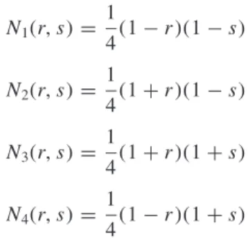
RECTANGULAR ELEMENTS
Using this reasoning, the interpolation function associated with node 1 must be of the form 4(r−1)(1+s)(r−s+1) (6.59d) The form of the interpolation functions associated with the center nodes is easier to obtain than that for the corner nodes.
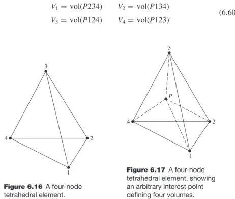
THREE-DIMENSIONAL ELEMENTS
- Four-Node Tetrahedral Element
A parallel procedure for the interpolation functions associated with the other three corner nodes leads to. The form of the interpolation functions associated with the middle nodes is easier to obtain than those for the corner nodes.