Optimal scheduling of thermal-wind-solar power system with storage S. Surender Reddy
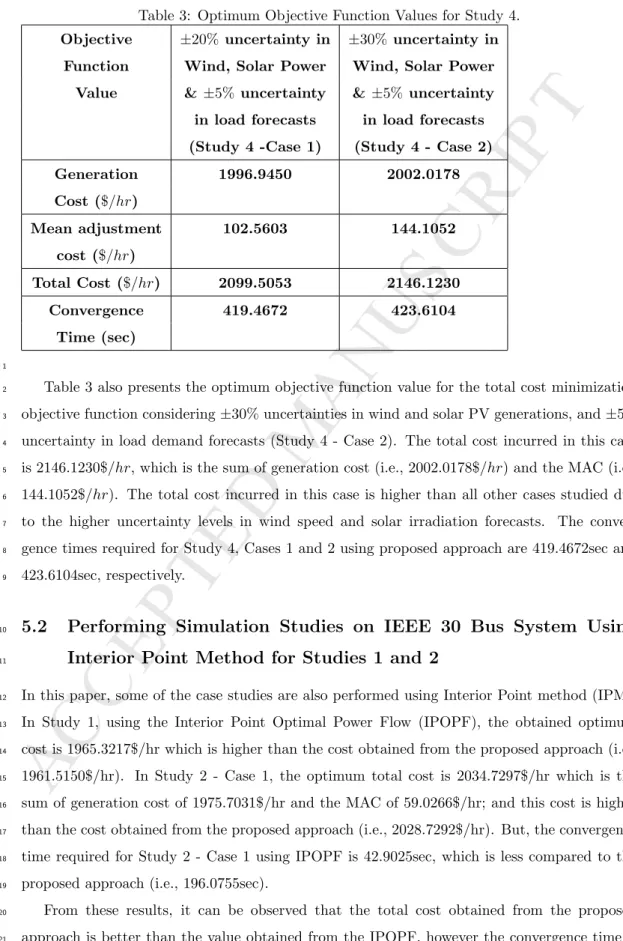
PII: S0960-1481(16)30887-4 DOI: 10.1016/j.renene.2016.10.022 Reference: RENE 8210
To appear in: Renewable Energy Received Date: 15 December 2015 Revised Date: 9 September 2016 Accepted Date: 12 October 2016
Please cite this article as: Reddy SS, Optimal scheduling of thermal-wind-solar power system with storage, Renewable Energy (2016), doi: 10.1016/j.renene.2016.10.022.
This is a PDF file of an unedited manuscript that has been accepted for publication. As a service to our customers we are providing this early version of the manuscript. The manuscript will undergo copyediting, typesetting, and review of the resulting proof before it is published in its final form. Please note that during the production process errors may be discovered which could affect the content, and all legal disclaimers that apply to the journal pertain.
M ANUS
CR IP T
AC CE PTE D
Optimal Scheduling of Thermal-Wind-Solar Power System
1
with Storage
2
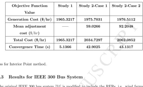
S. Surender Reddy
Department of Railroad and Electrical Engineering, Woosong University, Republic of Korea.
Ph: +82-426296735
Corresponding Author: [email protected]
3
Abstract
4
The incorporation of renewable energy resources (RERs) into electrical grid is very chal-
5
lenging problem due to their intermittent nature. This paper solves an optimal scheduling
6
problem considering the hybrid generation system. The primary components of hybrid
7
power system include conventional thermal generators, wind farms and solar photovoltaic
8
(PV) modules with batteries. The main critical problem in operating the wind farm or
9
solar PV plant is that these RERs cannot be scheduled in the same manner as conventional
10
generators, because they involve climate factors such as wind velocity and solar irradia-
11
tion. This paper proposes a new strategy for the optimal scheduling problem taking into
12
account the impact of uncertainties in wind, solar PV and load demand forecasts. The
13
simulation results for IEEE 30 and 300 bus test systems with Genetic Algorithm (GA) and
14
Two-Point Estimate Method (2PEM) have been obtained to test the effectiveness of the
15
proposed optimal scheduling strategy. Results for sample systems with GA and two-point
16
estimate based optimal power flow, and GA and Monte Carlo Simulation (MCS) have been
17
obtained to ascertain the effectiveness of proposed method. Some of the results are also
18
compared with the Interior Point method. From the simulation studies, it can be observed
19
that with a marginal increase in the cost of day-ahead generation schedule, a substantial
20
reduction in real time mean adjustment cost is obtained.
21
Index Terms: Energy Storage, Load Forecast Uncertainty, Optimal Scheduling, Renewable
22
Energy Resources, Solar Energy System, Wind Energy System.
23
1 Introduction
24
The integration of stochastic weather-driven power sources has resulted in larger uncertainties
25
that need to be met by dispatchable generation and storage. The concerns brewing up over
26
fossil fueled generating plants and their part of play in global warming has pushed energy based
27
M ANUS
CR IP T
AC CE PTE D
research towards utilization of green energy around the globe. With the greater incorporation of
1
renewable electricity generation like wind and solar photovoltaic (PV) power into the existing
2
grids, research efforts must be devoted to formulate generation scheduling problems taking
3
into account the intrinsic variability and non-dispatchable characteristics of these Renewable
4
Energy Resources (RERs). The random nature and large scale integration of renewable sources
5
into power system poses challenges to the system operators and/or planners. Solar irradiation
6
and wind velocity are uncertain and their availability is irrelevant the load variation. The
7
variability and intermittency of these resources creates important challenges to be overcome
8
in the generation scheduling problem. This intermittent nature may have negative effects on
9
the entire grid. One of the most viable solutions is the integration of energy storage, which
10
mitigates against fluctuations in generation and supply. Energy storage may improve power
11
management in the grid that include renewable energy resources. The storage devices match
12
energy generation to consumption, facilitating a smooth and robust energy balance within the
13
grid. However, this adds another degree of complexity to the generation scheduling.
14
The developments to the solar PV technology leads to lower manufacturing costs which
15
allows the solar PV power to occupy higher percentage of electric power generation in the near
16
future. In recent years, the grid connected solar PV system with battery storage is becoming
17
more popular because of its impact on the peak load reduction, to reduce the fluctuations of
18
renewable energy sources, congestion mitigation and pricing, and the commitment of expensive
19
thermal units. The energy storage allows to store the surplus solar electricity. During the day
20
(i.e., the solar PV system generates solar electricity), the battery storage system will ensure
21
that surplus energy is used to charge the battery or exported to the grid. In the evening or at
22
time of low solar PV generation, the battery system can discharge the stored electricity.
23
The operation of power systems has for a long time been informed by Optimal Power Flow
24
(OPF). OPF is used to dispatch available generation in such a way that minimizes a particular
25
objective function. OPF can fully represent the network and nodal power balance equations.
26
It also maintains limits on bus voltage, branch power flows, and generator’s active and reactive
27
power outputs [1]-[2]. The deregulation and restructuring of power system industry along with
28
mandates to incorporate Renewable Energy Resources (RERs) is introducing new challenges
29
for the power system. RERs, in particular, need mitigation strategies in order to maintain
30
reliable power on the electrical grid. The operational challenges associated with the integration
31
of RERs can be alleviated by effectively utilizing the grid-integrated distributed energy storage
32
[3]. The potential benefits of grid-integrated storage technologies include decreasing the need
33
for new transmission and/or generation capacity, improving load following, providing spinning
34
reserve, correcting frequency, voltage, and power factors, as well as the indirect environmental
35
advantages gained through facilitating an increased penetration of RERs [3].
36
This paper solves an optimal scheduling problem in a hybrid power system. The primary
37
M ANUS
CR IP T
AC CE PTE D
components of the hybrid system comprises the conventional thermal generators, wind farms
1
and solar PV plants. A set of batteries is available for the energy storage and/or discharge. The
2
important problem in operating a wind farm or solar PV plant is that RERs cannot be scheduled
3
in the same manner as conventional generators, because they involve climate factors eg. wind
4
velocity and solar irradiation. The wind velocity and solar irradiation are uncertain and their
5
availability is irrelevant to the load demand variation. The variability and intermittency of the
6
resources are important challenges to be overcome in the generation dispatching/scheduling.
7
Wind and solar PV power generations have very high uncertainty and variability.
8
Solar power is growing at a very rapid clip. Total global solar PV capacity is fast approaching
9
the 100GW milestone, according to a new report from the International Energy Agency [4].
10
The report notes that even with some uncertainty present about the future state of PVs in
11
the European and Chinese markets, that global installed capacity will almost definitely hit
12
the 100GW milestone within the year. PV technologies instantaneously convert the irradiance
13
into electricity, this change in irradiance causes immediate changes in power generation. For
14
wind power technology, it is right way to classify as variable output power source instead of
15
variable/intermittent source, because the power output does not stop and start on the basis of
16
minute-to-minute time scale. For solar PV plants, the term variable fits well, because cloud
17
shadowing can abruptly change the power production. On the second to minute time scale,
18
conflicting to wind power, solar PV power can have a strong effect on the reserves. Even a clear
19
day, without the effect of cloud shadows, for sunrise and sunset, the solar based electric power
20
varies 80% in 1 hour, instantaneously, for all solar PV power generation in the system.
21
An optimal scheduling approach for the wind-solar-storage generation system considering
22
the correlation among wind power output, solar PV power output and load demand is proposed
23
in [5]. The optimal control/management of Microgrid’s energy storage devices is addressed in
24
[6]. The traditional OPF problem without storage is a static optimization problem as there is a
25
need to balance generation and demand at all the times decouples the optimization in different
26
time periods. The inclusion of storage introduces correlation and an opportunity to optimize,
27
across the time, e.g., the cost of generation is inversely proportional to discharge [7]. In [8], an
28
AC-OPF simulation results are used to study the effects of large-scale energy storage systems
29
on the power system. The economic effects are also analyzed under several different operating
30
conditions, andCO2 emission reductions offered by the use of storage are considered.
31
A stochastic model of wind generation in OPF problem is addressed in [9]. The model
32
includes error in wind power generation forecasts using probability or relative frequency his-
33
togram. A robust DC-OPF for a smart grid with high penetration of wind generation is pro-
34
posed in [10]. Here, the optimal dispatch is obtained as the solution to a convex program with
35
a suitable regularizer, which is able to mitigate the potentially high risk of inadequate wind
36
power. In [11], a risk mitigating OPF framework to study the placement and dispatch of energy
37
M ANUS
CR IP T
AC CE PTE D
storage units in power system with wind power generators that are supplemented by conven-
1
tional fast-ramping back-up generators is proposed. In [12], a probabilistic model of Security
2
Constrained Unit Commitment (SCUC) is proposed to minimize the cost of energy, spinning
3
reserve and possible loss of load. Reference [13] proposes a solution strategy that uses a convex
4
optimization based relaxation to solve the optimal control problem. Reference [14] proposes
5
the problem of coordinating wind-thermal power system using OPF model. The uncertainty
6
caused by wind power generation has two-fold effect as wind power spillage and deficit that
7
both of them are stated in terms of cost. These costs are considered as extra costs to manage
8
wind intermittency.
9
A two-stage stochastic version of classical economic dispatch problem with AC power flow
10
constraints, a non-convex optimization formulation that is central to power transmission and
11
distribution over an electricity grid is proposed in [15]. Reference [16] introduces the Chance
12
Constrained Programming (CCP) approach to OPF under uncertainty and analyze the com-
13
putational complexity of the chance constrained OPF. The effectiveness of implementing a
14
back-mapping approach and a linear approximation of the non-linear model equations to solve
15
the formulated CCP problem is investigated in this paper. Reference [17] proposes a problem
16
formulation which minimizes the average cost of generation over the random power injections,
17
while specifying a mechanism by which generators compensate in real-time for renewable power
18
fluctuations; at the same time guaranteeing low probability that any line will exceed its rating.
19
Reference [18] builds the lowest-cost optimization model, considering the investment, operating
20
costs of system and environmental governance as well as two operation modes, isolated and
21
grid-connected operation, and proposes the scheduling strategy of the hybrid generation, with
22
the aim to realize the best configuration of output power of the RERs.
23
A comprehensive review of various aspects of hybrid renewable energy system including the
24
pre-feasibility analysis, optimum sizing, modeling, control aspects and reliability issues is pre-
25
sented in [19]. A short-term optimal operation scheduling of a power generation company with
26
integrated wind and storage is presented in [20]. An optimal day-ahead scheduling approach
27
for the integrated urban energy system is introduced in [21], which considers the reconfigurable
28
capability of an electric distribution network. Reference [22] proposes a novel interval optimiza-
29
tion based day-ahead scheduling model considering renewable energy generation uncertainties
30
for the distribution management systems. A new risk-constrained two-stage stochastic program-
31
ming model to make optimal decisions on energy storage and thermal units in a transmission
32
constrained hybrid wind-thermal power system to control the risk of the operator decisions is
33
presented in [23]. Reference [24] proposes a model to minimise the hybrid system’s operation
34
cost while finding the optimal power flow considering the intermittent solar and wind resources,
35
the battery state of charge and the fluctuating load demand. Reference [25] proposes the opti-
36
mal scheduling strategy taking into account the impact of uncertainties in wind, solar PV, and
37
M ANUS
CR IP T
AC CE PTE D
load forecasts, and provides the best-fit day-ahead schedule by minimizing both day-ahead and
1
real-time adjustment costs including the revenue from renewable energy certificates.
2
From the above literature review, it can be observed that there is no optimal scheduling
3
approach, which will handle the uncertainties in wind, solar PV and load demand including
4
battery storage mechanism. In view of the uncertainties involved in wind power, solar PV power
5
generation and load demand forecast, day-ahead (DA) scheduling strategies need to adapt to
6
these requirements approximately. In this regard, some attempts have been made in the litera-
7
ture, but a methodology which can clearly reflect the cost implications of the differences in the
8
DA schedule, and the real-time (RT) dispatch is required. This paper is aimed at bridging this
9
gap. In the proposed optimal scheduling strategy, the uncertainties in wind, solar PV power
10
generation and/or load demands are handled by the power system operator (SO) using the
11
anticipated real time (RT) adjustment bids. Since, the market clearing is a multi-settlement
12
process: day-ahead and real time, a strategy is proposed that provides the ‘best-fit’ day-ahead
13
schedule, which minimizes the twin (both day-ahead and real time adjustment) costs, under all
14
possible scenarios in real time. This two stage optimization strategy consists of a genetic algo-
15
rithm (GA) based day-ahead optimum scheduling and a two-point estimate based probabilistic
16
real time optimal power flow (RT-OPF). The former generates sample schedules with respect
17
to which, the latter provides mean adjustment costs. Our proposed model characterizes the
18
structure of optimal power generation and charge/discharge schedule.
19
The remainder of the paper is organized as follows: Section 2 presents the problem formu-
20
lation and the proposed solution methodology for optimal scheduling with Renewable Energy
21
Resources (RERs) including storage. Section 3 presents the uncertainty modeling of wind en-
22
ergy system. Section 4 describes the solar energy system, and the uncertainty modeling of
23
solar energy system and load demand. Section 5 presents the simulation results and discussion.
24
Finally, the contributions with concluding remarks are presented in Section 6.
25
2 Optimal Scheduling with RERs and Storage: Problem
26
Formulation
27
In this paper, an optimal scheduling problem is formulated and solved considering the thermal-
28
wind-solar hybrid generation system. The primary components considered for the hybrid power
29
system are conventional thermal generators, wind farms and solar PV modules with batteries.
30
The problem proposed in this paper is suitable for the large grid. The optimal scheduling with
31
RERs and storage is very important for the optimal operation and planning of power systems to
32
address the variability and uncertainty associated with increasing renewable power generation.
33
The output of solar PV array/wind turbine is predicted according to the weather forecast. As
34
the input energy of wind power generation (wind) and solar power generation (sun) is uncertain,
35
M ANUS
CR IP T
AC CE PTE D
the output of these resources is also uncertain. Normally, the probability distribution function
1
is used to model the related uncertainty.
2
In this paper, it is considered that wind and solar PV power generations can be sched-
3
uled/dispatched, and can bid in the electricity market. However, the system operator should
4
consider appropriate amount of spinning reserves in the operational plan. The required amount
5
of spinning/non-spinning reserves can be calculated using Probability Density Function (PDF)
6
of wind and solar PV power generation [26]-[28]. This paper presents the optimal scheduling
7
strategy of wind and solar PV power generators in the OPF module. In this paper, an optimal
8
scheduling strategy for the integrated operation of thermal, wind power and solar PV modules
9
in the centralized power market is proposed. The objective function is formulated as,
10
Minimize,
11
NG
X
i=1
CGi(PGi) +
NW
X
j=1
CW j(PW j) +
NS
X
k=1
CSk(PSk) +
NG
X
i=1
CRT i(PgDev,i) (1) whereNG,NW andNS are the number of thermal, wind and solar PV generators, respectively.
12
The terms in the objective function (i.e., Eq. (1)) are described next:
13
The first term in Eq. (1) is the fuel cost of conventional thermal generators, and it is
14
expressed as,
15
CGi(PGi) =ai+biPGi+ciPGi2 (2) where PGi is the scheduled power output from ith conventional thermal generator in MWs,
16
CGi(PGi) is the fuel cost function of conventional thermal generators, andai,bi, andciare the
17
fuel cost coefficients ofith conventional thermal generating unit.
18
In the objective function (i.e., Eq. (1)), the second term is the direct cost given to wind plant
19
owner for the scheduled wind power. In the case where the wind/solar PV plants are owned
20
by the system operator, the cost function may not exist as the wind/solar PV power requires
21
no fuel, unless the system operator wants to assign some payback cost to the initial outlay for
22
the wind/solar PV plants or unless the system operator wants to assign this as a maintenance
23
and renewal cost [29]. But, in a non-utility owned wind/solar PV plants, the wind/solar PV
24
generation will have a cost that must be based on the special contractual agreements. The
25
output of the wind/solar PV generator is constrained by an upper and lower limit, decided by
26
the system operator based on the agreements for the optimal operation of the system [30]. For
27
simplicity, this can be considered to be proportional to the scheduled wind/solar PV power
28
or totally neglected [9], [31]. Therefore, the cost is neglected in the system-operator-owned
29
wind/solar PV plants, and considered to be proportional to the scheduled wind/solar PV power
30
for the non-utility-owned wind/solar PV plants. In this paper, a linear cost function is used for
31
the scheduled wind power [32]-[33], and it is expressed as,
32
CW j(PW j) =djPW j (3)
M ANUS
CR IP T
AC CE PTE D
where PW j is the scheduled wind power generation from jth wind farm in MWs, CW j(PW j)
1
is the cost function of wind energy generator, and dj is the direct cost coefficient ofjth wind
2
farm/generator.
3
The third term is the direct cost for the scheduled solar PV power. As explained earlier, a
4
linear cost function is used for the scheduled solar PV power, and it is expressed as [34],
5
CSk(PSk) =tkPSk (4)
wherePSkis the power output fromkthsolar PV plant (MW), andtkis the direct cost coefficient
6
ofkth solar PV plant.
7
The fourth term in Eq. (1) is the mean adjustment cost (MAC), which accounts the cost
8
due to uncertain nature of wind, solar PV power and load demand. In real time (RT), thermal
9
generators deviate from their day-ahead (DA) schedules due to uncertain nature of wind velocity,
10
solar irradiation and load demand forecast. This deviation power is the difference between day-
11
ahead scheduled power (PGiDA), and uncertain real time power (PgGiRT). A quadratic real time
12
adjustment cost function is used to calculate the mean adjustment cost (MAC), and is given by
13
CRT i(PgDev,i) =CRT i(|PGiDA−PgGiRT|)
14
=xi+yiPgDev,i+ziPgDev,i
2 (5)
wherePDev,i is the deviation power fromithconventional thermal generator. xi,yi andzi are
15
the cost coefficients ofithconventional thermal generator in real-time.
16
2.1 Equality and Inequality Constraints
17
The equality and inequality constraints for the above problem are presented next:
18
2.1.1 Nodal Power Balance Constraints
19
The power balance constraints include active and reactive power balances. The power flow
20
equations reflect the physics of the power system as well as the desired voltage set points
21
throughout the system. The physics of the power system are enforced through the power flow
22
equations which require the net injection of active and reactive power at each bus sum to zero.
23
The sum of power generated by conventional thermal generators, wind farms and solar PV
24
modules is equal to the sum of the total demand and losses in the system.
25
Pi=Vi
n
X
j=1
[Vj[Gijcos(δi−δj) +Bijsin(δi−δi)]]−PGi−PDi (6)
26
Qi=Vi n
X
j=1
[Vj[Gijsin(δi−δj)−Bijcos(δi−δi)]]−QGi−QDi (7)
M ANUS
CR IP T
AC CE PTE D
where
1
PGi=
NG
X
j=1
PGj+
NW
X
k=1
PW k+
NS
X
l=1
PSl (8)
PDi and QDi are the load active and reactive power, respectively. Yij = Gij +jBij is the
2
ijth entry of the nodal admittance matrix. Gij and Bij are the transfer conductance and
3
susceptance between busiand busj, respectively.
4
2.1.2 Generator Constraints
5
The power output of each thermal generator is restricted by their minimum, maximum limits
6
and generator rate constraints (GRC).
7
max[PGimin, PGi0 −RdownGi ]≤PGi≤min[PGimax, PGi0 +RupGi] (9) The power output of each wind generator is restricted by,
8
0≤Pwj≤Prj j= 1,2, ..., NW (10)
wherePrj is submitted as part of the wind producer energy offer. In DA scheduling, the wind
9
power (Pwj) varies in the following range
10
0≤Pwj≤Pwf,j j= 1,2, ..., NW (11) wherePwf,j is the forecasted wind power fromjthwind generator, which is obtained from the
11
forecasted wind speed.
12
The maximum penetration of solar PV to system is given by,
13
|PSk| ≤PSkmax k= 1,2, ..., NS (12) where PS (MW) is the solar PV active power generation (unknown), and PSmax (MW) is the
14
available maximum active power generation (known) subject to solar irradiation and temper-
15
ature. PS can be positive or negative. A positive PS indicates that power flow from the PV
16
plant to the utility/grid. A negative PS indicates that power flow from the grid to the solar
17
energy system, this is due to the charging of the batteries during the off-peak period.
18
Generator voltage magnitudes (VG), generator reactive power (QG) are restricted by their
19
lower and upper limits [35]-[38], and they are represented by
20
VGimin≤VGi≤VGimax i(NG+NW +NS) (13)
21
QminGi ≤QGi≤QmaxGi i(NG+NW +NS) (14)
M ANUS
CR IP T
AC CE PTE D
2.1.3 Security Constraints
1
These constraints include the limits on load bus voltage magnitudes (VDi), line flow limits (Sij)
2
and transformer tap (T Tt) constraints [39].
3
VDimin≤VDi≤VDimax i= 1,2, ..., Nl (15)
4
|Sij| ≤Sijmax (16)
5
T Ttmin ≤T Tt≤T Ttmax t= 1,2, ..., NT (17) whereNlis the number of load demands,Sij is MVA (mega-volt ampere) flow andSijmaxis the
6
maximum thermal limit of line between busi and busj. T Tt is transformer tap settings and
7
NT is number of transformer taps.
8
2.2 Proposed Solution Methodology
9
For a specified day-ahead (DA) schedule, one can not know what exactly the actual real time
10
(RT) conditions would be. In order to accommodate these changes, a real time optimal power
11
flow (RT-OPF) problem is solved by using adjustment bids supplied by the market participants.
12
However, while optimizing the DA schedule, one does not know, what will be the RT condition.
13
Hence, a probabilistic OPF (P-OPF) with the uncertainty data given, appears to be a good
14
option. The difference in the DA and RT schedules can be used to evaluate the mean adjustment
15
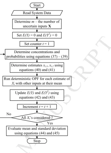
cost (MAC). The proposed solution approach/procedure is shown in Figure 1. This figure
16
depicts the two stage optimal scheduling strategy including day-ahead optimal power flow (DA-
17
OPF) and probabilistic RT-OPF. The MAC is calculated using probabilistic RT-OPF. This
18
probabilistic RT-OPF is solved inside the DA-OPF module. The inputs to the proposed optimal
19
scheduling module are the system/network data and forecasts data of wind power, solar PV
20
power and load demand. From Figure 1, it can be observed that the day-ahead schedules can
21
be observed from Genetic Algorithm (GA) and the real time (RT) schedules can be determined
22
by using Two-point estimate based RT-OPF. By using these DA and RT schedules, the MAC
23
can be calculated. Then the objective function is formulated using the generation costs of
24
thermal generators, wind farms, solar PV plants and the MAC. In order to determine the
25
optimal decision variables, to optimize an objective function and to satisfy the constraints, the
26
variables are to be represented in the binary strings. The description about representation
27
and encoding of chromosome (i.e., overview of GA) is presented in [40]. The fitness function
28
evaluation is presented in [41].
29
Corresponding to a given DA generation schedule, the MAC is evaluated over the uncertainty
30
range of wind, solar PV and load demand forecast using P-OPF. Therefore, obtaining the
31
analytical expression of this cost, in terms of the DA schedule variables, is difficult. Because
32
of this, it is difficult to use the gradient based optimization techniques to solve this problem.
33
M ANUS
CR IP T
AC CE PTE D
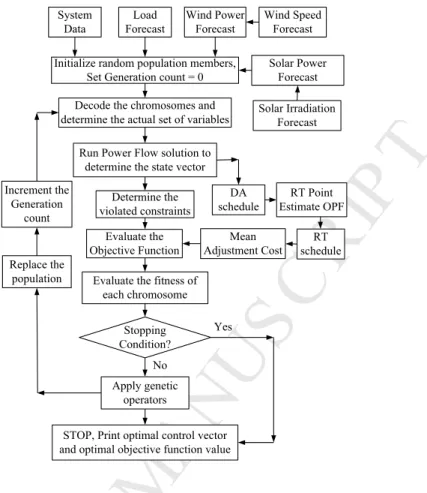
Figure 1: Flow Chart of Solution Procedure for Optimal Scheduling with RERs and Storage.
Hence, in this paper, we used evolutionary/meta-heuristic optimization techniques to get the
1
DA schedules.
2
Here, genetic algorithm (GA) is used to solve this optimal scheduling with RERs and storage
3
problem. In the first stage i.e., in outer loop, GA is used to get the DA schedules. RT schedules
4
are obtained by using the probabilistic Two Point Estimate Method (2PEM), which is solved
5
in the inner loop. Using the DA schedules and RT schedules, the deviation power (PDev,i) is
6
calculated. PDev,iis the difference between DA scheduled power and uncertain RT power. The
7
MAC is calculated by considering the real time adjustment bids. After calculating the MAC,
8
the objective function is formulated and is optimized using GA [40]. The RT schedules are
9
obtained using P-OPF to account for the uncertainties involved due to wind, solar PV power
10
generations and load demand forecasts. Since, OPF basically being a deterministic tool, it
11
has to run several times to encompass all possible operating conditions. More accurate Monte
12
Carlo Simulation (MCS) methods, which will handle complex random variables, provide an
13
alternative, but MCS is computationally more demanding. Therefore, here an efficient 2PEM
14
based P-OPF is used.
15
In order to account for the uncertainties in proposed optimal scheduling problem, a two-
16
point estimate method (2PEM) [42] is used. Both MCS and 2PEM use deterministic routines
17
M ANUS
CR IP T
AC CE PTE D
for solving the probabilistic problems; but, the latter requires a much lesser computational
1
burden. The 2PEM overcomes difficulties associated with the lack of perfect knowledge of the
2
probability functions of stochastic variables, since these functions are approximated using only
3
their first few statistical moments (i.e., mean, variance, skewness, and kurtosis). Therefore, a
4
smaller level of data is required [43]. This method needs 2m runs of deterministic OPF form
5
uncertain variables, and it does not require derivatives of the non-linear function used in the
6
computation of probability distributions. The description of 2PEM is presented in Appendix
7
A.
8
2.3 Real Time Optimal Power Flow (RT-OPF) Model
9
Probabilistic RT-OPF is used to calculate the mean adjustment cost (MAC), and the two-point
10
estimate OPF is used to solve this RT-OPF problem. This two-point estimate method (2PEM)
11
uses deterministic OPF. The deterministic and probabilistic RT-OPF models are formulated
12
next:
13
2.3.1 Deterministic RT-OPF Model
14
In this model, the objective is to minimize the deterministic mean adjustment cost (MAC), and
15
is formulated as,
16
minimize
NG
X
i=1
CRT i(PDev,i) =
NG
X
i=1
CRT i(|PGiDA−PGiRT|) (18) Subjected to equality and inequality constraints presented in Section III-A.
17
2.3.2 Probabilistic RT-OPF Model
18
In this model, the objective is to minimize the MAC due to uncertainty in wind generation,
19
solar PV power and load demand forecasts. For probabilistic RT-OPF, the uncertain random
20
variable isPGiRT due to uncertainties in wind generation, solar PV power and load demand at
21
real time. Hence, Eq. (18) becomes
22
minimize
NG
X
i=1
CRT i(PgDev,i) =
NG
X
i=1
CRT i(|PGiDA−PgGiRT|) (19)
wherePgGiRT is a random variable. Subjected to equality and inequality constraints presented in
23
Section III-A. This problem is solved using two-point estimate OPF [44].
24
In real time (RT), if the scheduled wind power (PW j) varies in±x%, then
25
Pmaxmin=PW f,j− x
100×PW f,j
(20) and
26
Pmaxmax=PW f,j+ x
100 ×PW f,j
(21)
M ANUS
CR IP T
AC CE PTE D
Therefore, in real time optimal power flow (RT-OPF),
1
Pmaxmin≤Pmax≤Pmaxmax (22)
2
0≤Pwj ≤Pmax (23)
and the similar expressions are valid for solar PV power generation also.
3
In order to account for uncertainties in the day-ahead optimal scheduling, a Two-Point
4
Estimate Method (2PEM) [42] is used. Both Monte Carlo simulation (MCS) and 2PEM use
5
deterministic routines for solving probabilistic problems [43, 44]; however, the latter requires a
6
much lower computational burden.
7
3 Wind Energy System
8
In order to incorporate the RERs in the optimal scheduling problem, some characterization of
9
the uncertain nature of wind speed, solar irradiation and load demand are needed. An important
10
barrier to the incorporation of the wind power into the electrical grid is its variability. Various
11
probability distribution functions are proposed for the statistical analysis of recorded wind
12
speeds. Here, Weibull Probability Density Function (PDF) is used for the wind speed and
13
then, transformed to the corresponding wind power distribution for use in proposed optimal
14
scheduling model. The wind power output will follow stochastic nature as compared to the
15
wind speed [45]-[46].
16
For a given wind speed input, the wind power output [9], [31] is expressed as,
17
p=
0 forv < viand v > v0 pr
v−vi
vr−vi
forvi≤v≤vr pr forvr≤v≤v0
(24)
wherepis power output of wind energy generator in MWs,vis the wind speed (in m/sec), and
18
vi, vo, vrare the cut-in, cut-out and rated wind speeds, respectively.
19
3.1 Uncertainty Modeling of Wind Energy System
20
The wind speed is modeled by using Weibull Probability Density Function (PDF), and is
21
expressed as [31],
22
f(v) = k
c v
c k−1
exp
−v c
k
0< v <∞ (25) For the Weibull PDF (i.e., Eq. (25)), the corresponding Cumulative Distribution Function
23
(CDF) is expressed as [47],
24
FV(v) = 1−exp
−v c
k
(26) If it is assumed that the wind speed has a given distribution, such as the Weibull, it is then
25
necessary to convert that distribution to a wind power distribution. This transformation may
26
M ANUS
CR IP T
AC CE PTE D
be accomplished in the following manner, with V as the wind speed random variable and P
1
as the wind power random variable. For a linear transformation, in general [31], such as that
2
described in Eq. (24)
3
P =T(V) =aV +b (27)
and
4
fP(p) =fV[T−1(p)]
dT−1(p) dp
=fV
p−b a
1 a
(28) The wind generation output in the continuous range (vi≤v≤vr) is given by [31], [47],
5
p=pr
v−vi
vr−vi
= pr
vr−vi
v−
vi
vr−vi
(29) wherea= (vpr
r−vi) andb=−(vvi
r−vi).
6
According to the theory for function of random variables, Eq. (28) will take the form,
7
fP(p) = khvi
prc
1 +hpp
rvi
c
(k−1)
×exp
−
1 +hpp
rvi
c
k
(30)
where h=
vr
vi
−1 is an intermediary parameter. In this paper, the wind power output
8
in discrete range [31] is also considered. The sum of the probability of discrete and continuous
9
function is 1.
10
4 Solar Energy System
11
For the generation scheduling and dispatch, electric power utilities are interested in the avail-
12
ability of solar PV power on an hourly basis. The hourly meteorological data are required to
13
simulate the performance of solar energy. The actual size of the battery depends on amount of
14
peak shaving desired.
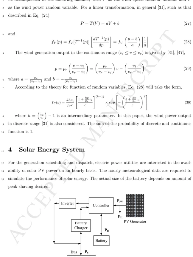
Figure 2: Solar Energy System Connected to Solar PV System With Battery Storage.
15
M ANUS
CR IP T
AC CE PTE D
In the presence of battery storage, the power output of solar PV cell (PP V) and the power
1
output of solar energy system (PS) are different. The power balance in solar energy system is
2
represented as [48],
3
PS=PP V(G) +PB−PU (31)
In this paper, we assume that there is no spillage power (PU(MW)) from PV. We also ignore the
4
effect of spillage power of the aggregated battery. The solar PV power output can be controlled
5
by the power tracking control scheme or to be charged into the batteries. Hence, the maximum
6
penetration of solar PV to system is given by [48]-[49],
7
|PS| ≤PSmax (32) In this paper, it is assumed that the battery voltage keeps constant during the scheduling pe-
8
riod (i.e., 1 hour). The maximum charge and discharge capacity of battery is represented by Eq.
9
(33). However, this limit depends on the rating of the battery. PBis the power charge/discharge
10
to/from battery (MW).PB is positive for discharging and negative for charging.
11
PB ≤PB ≤PB (33)
wherePB is the aggregated discharging power limit (positive) for all batteries (MW), andPB is
12
the aggregated charging power limit (negative) of all batteries (MW). In this paper, we ignore
13
the effect of spillage power of the aggregated battery.
14
IfCinitandCare aggregated battery state of charge of all batteries (kAh) at the beginning
15
and the end of the scheduling period (say 1 hour). The contribution of solar PV module to the
16
grid during interval ‘∆t’ (1 hour) is [48],
17
PS=PP V(G) +(Cinit−C)VB
ηB∆t −PU (34)
whereVB is battery voltage,ηB is the efficiency during the charging period (75%), andPP V(·)
18
is the solar irradiation to energy conversion function of the solar PV generator or power output
19
from solar PV cell [48], and is given by
20
PP V(G) =
Psr
G2 GstdRc
for 0< G < Rc
Psr
G Gstd
forG > Rc
(35)
In this paper, it is assumed that the solar PV cell temperature is ignored. Where,
21
G: Solar irradiation forecast inW/m2.
22
Gstd : In the standard environment, the solar irradiation is set as 1000W/m2.
23
Rc : A certain irradiation point set as 150W/m2.
24
Psr : Rated equivalent power output of the solar PV generator.
25
PB : Power charge/discharge to/from the battery.
26
M ANUS
CR IP T
AC CE PTE D
4.1 Uncertainty Modeling of Solar PV System
1
The power output of solar PV generator is mainly depends on irradiance. The distribution of
2
hourly irradiance at a particular location usually follows a bi-modal distribution, which can be
3
considered as a linear combination of two uni-modal distributions. The uni-modal distribution
4
functions can be modeled by Weibull, Beta and Log-normal PDFs. In this paper, the Weibull
5
probability distribution function is used and it is expressed as,
6
fG(G) =ω k1
c1 G c1
k1−1
exp
"
− G
c1 k1#
7
+(1−ω) k2
c2
G c2
k2−1
exp
"
− G
c2
k2#
0< G <∞ (36) where ω is weight parameter in the range between 0 and 1 (0< ω <1). k1,k2 and c1,c2 are
8
the shape and scale factors, respectively.
9
4.2 Normal Distribution for Load Demand Uncertainty
10
The future system load demand is uncertain at any given period of time. Normally used two
11
probability density functions (PDFs) for modeling load demand uncertainty are Normal and
12
Uniform PDFs. In this paper, Normal PDF is used to model the load distribution. The PDF
13
of normal distribution for uncertain load ‘l’ is given by [50],
14
fl(l) = 1 σL√
2Π×exp
−
(l−µL)2 2σL2
(37) whereµL andσL are the mean and standard deviation of the uncertain load, respectively.
15
5 Simulation Results and Discussion
16
IEEE 30 and 300 bus test systems [51] are used to establish the effectiveness of the proposed
17
optimal scheduling approach considering the Renewable Energy Resources (RERs) and storage.
18
5.1 Results for IEEE 30 Bus System
19
The original IEEE 30 bus test system is modified to include the RERs. The modified IEEE
20
30 bus system consists of 6 generators, among them 4 are considered as conventional thermal
21
generators located at the buses 1, 2, 5 and 8; and 2 are considered to be RERs, located at the
22
buses 11 and 13. A wind energy system is assumed at bus 11, and a solar energy system is
23
assumed at bus 13. The cost coefficients and generator power limits data of thermal, wind and
24
solar PV generators have been presented in Appendix B.
25
In IEEE 30 bus system, the maximum power limit of wind energy generator is considered
26
as 45MW. Here, we have assumed the forecasted wind velocity as 10m/sec. For a given wind
27
M ANUS
CR IP T
AC CE PTE D
speed forecast, the wind power output is determined using Eq. (24). Therefore, the wind
1
power output is 35MW i.e., from the system optimization point of view, the scheduled wind
2
power generation can go any where from 0 to 35MW, provided if there is no uncertainty in
3
the wind generation. Suppose, if we consider the uncertainty in wind power generation, then
4
the maximum power generation limits are differed by uncertainty margin (using Eq. (22)).
5
For the Two Point Estimate Method (2PEM), the samples are generated between Pmaxmin and
6
Pmaxmax, which will follow Weibull PDF. Weibull PDF is assumed to represent the wind speed,
7
and then it is transformed to the corresponding wind power distribution, which can be used in
8
the proposed optimal scheduling problem.
9
The maximum power generation limit of solar PV system is considered as 40MW. Here, we
10
have assumed the forecasted irradiation as 500 W/m2. For a given solar irradiation forecast,
11
the solar PV power output is calculated using Eq. (35). Therefore, the solar PV power output
12
(i.e., PP V(G)) is 20MW. Bi-modal distribution function is used to represent the uncertainty
13
in solar PV power generation. The minimum and maximum limits of State of Charge (SOC)
14
of the battery are considered as 5kAh and 15kAh, respectively. The initial SOC is assumed
15
to be 10kAh. The efficiency of the battery and inverter are 75% and 95%, respectively. The
16
uncertainty levels of wind, solar PV power and load demand forecasts depends on the historical
17
data and their probability analysis (i.e., mean, standard deviation, etc). In this paper, we have
18
considered ±20% and±30% uncertainty for wind and solar PV plants; and±5% uncertainty
19
for load demands based on the historical wind speed, solar irradiation and load demand data
20
given in [52].
21
In recent years, MATLAB software has been used successfully for solving the power system
22
optimization problems [53]-[58]. In this paper, all the optimization programs are coded in
23
MATLAB and are implemented on a PC-Core 2 Quad Computer with 8GB of RAM. The
24
simulation results for different case studies on IEEE 30 bus system are presented next:
25
5.1.1 Study 1: Optimizing total cost minimization objective function with no un-
26
certainties in wind, solar PV power generations, and load demand forecasts
27
Generally, the cost of wind and solar PV power generations are lesser than the conventional
28
thermal generation costs. Therefore, they tends to schedule to their maximum forecasted power
29
output. However, for security reasons the OPF program can curtail their power output. This
30
case does not consider any uncertainties in wind, solar PV power generations and demand
31
forecasts. In this case, the total cost minimization objective function consists only first 3
32
terms of Equation (1), i.e., costs due to conventional thermal generators, wind farms and
33
solar PV plants. The scheduled power outputs of wind farm and solar PV plant located at
34
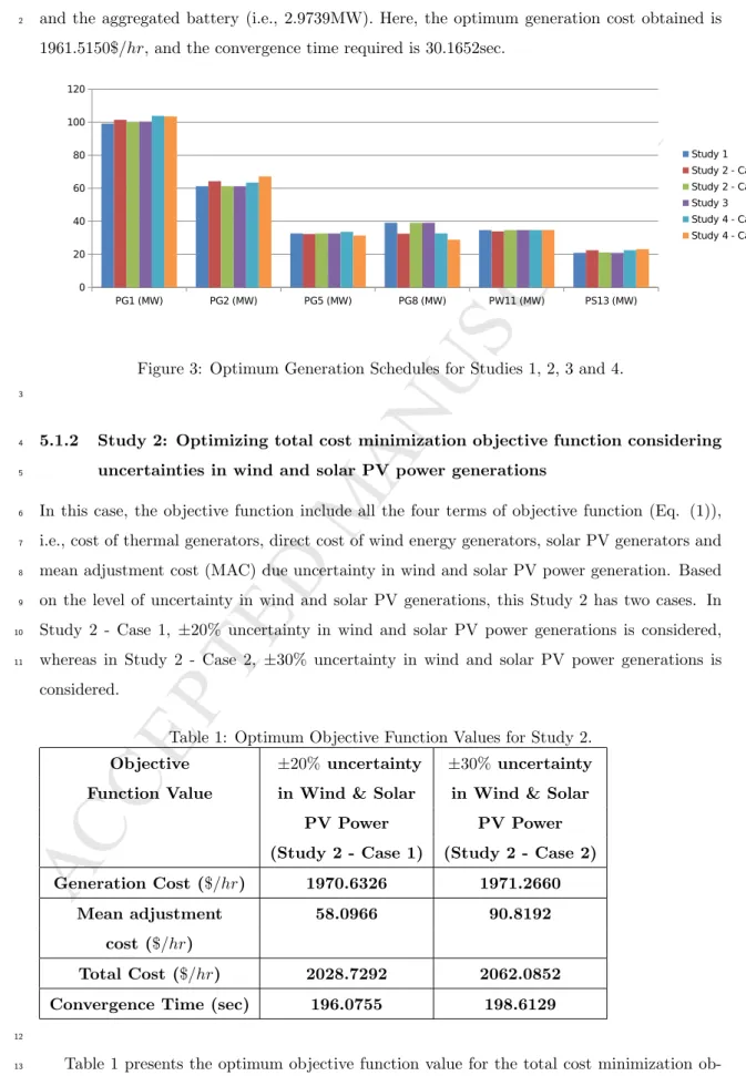
buses 11 and 13 are 34.6752MW and 20.9207MW, respectively. Figure 3 depicts the optimum
35
generation schedules for Studies 1, 2, 3 and 4. The power generated from the solar PV system
36
M ANUS
CR IP T
AC CE PTE D
(i.e., 20.9207MW) is the sum of power generated from solar PV generator (i.e., 17.9468MW)
1
and the aggregated battery (i.e., 2.9739MW). Here, the optimum generation cost obtained is
2
1961.5150$/hr, and the convergence time required is 30.1652sec.
Figure 3: Optimum Generation Schedules for Studies 1, 2, 3 and 4.
3
5.1.2 Study 2: Optimizing total cost minimization objective function considering
4
uncertainties in wind and solar PV power generations
5
In this case, the objective function include all the four terms of objective function (Eq. (1)),
6
i.e., cost of thermal generators, direct cost of wind energy generators, solar PV generators and
7
mean adjustment cost (MAC) due uncertainty in wind and solar PV power generation. Based
8
on the level of uncertainty in wind and solar PV generations, this Study 2 has two cases. In
9
Study 2 - Case 1, ±20% uncertainty in wind and solar PV power generations is considered,
10
whereas in Study 2 - Case 2, ±30% uncertainty in wind and solar PV power generations is
11
considered.
Table 1: Optimum Objective Function Values for Study 2.
Objective ±20% uncertainty ±30% uncertainty Function Value in Wind & Solar in Wind & Solar
PV Power PV Power
(Study 2 - Case 1) (Study 2 - Case 2) Generation Cost ($/hr) 1970.6326 1971.2660
Mean adjustment 58.0966 90.8192
cost ($/hr)
Total Cost ($/hr) 2028.7292 2062.0852 Convergence Time (sec) 196.0755 198.6129
12
Table 1 presents the optimum objective function value for the total cost minimization ob-
13
M ANUS
CR IP T
AC CE PTE D
jective with ±20% uncertainty in wind and solar PV power generation (i.e., Study 2 - Case
1
1). The obtained optimum scheduled power outputs for this study are depicted in Figure 3.
2
For the wind farm located at bus 11, the scheduled wind power is 33.9060MW, and for the
3
solar PV plant located at bus 13, the scheduled solar PV power is 22.4843MW. The scheduled
4
power output from the solar PV module is the sum of power generated from solar PV plant
5
(i.e., 18.2762MW) and the aggregated battery storage (i.e., 4.2081MW). In this Study 2 - Case
6
1, the optimum total cost obtained is 2028.7292 $/hr, which includes thermal, wind and solar
7
PV generation cost of 1970.6326 $/hrand mean adjustment cost (MAC) of 58.0966 $/hr. The
8
total cost incurred in this case is higher than cost obtained from the Study 1, due to ±20%
9
uncertainty in wind and solar PV power generation.
10
The results obtained in this Study 2 - Case 1 are also validated using MCS. The mean
11
adjustment cost obtained from MCS (10000 samples) with ±20% uncertainty in wind and
12
solar PV power generation is 58.0893 $/hr, and hence the total cost is 1970.6326 + 58.0893 =
13
2028.7219$/hr, which is approximately equal to total cost (2028.7292 $/hr) obtained from the
14
proposed approach considering two-point estimate method (2PEM).
15
Suppose, if we consider the schedules of Study 1 and calculating the MAC with ±20%
16
uncertainty in wind and solar PV power generation then the obtained MAC is 109.1132 $/hrand
17
generation cost same as Study 1, i.e., 1961.5150 $/hr. Therefore, the total cost is 1961.5150 +
18
109.1132 = 2070.6282$/hr, which is higher than the cost obtained in Study 2 - Case 1, i.e.,
19
2028.7292 $/hr, even though the ‘best-fit day-ahead schedule’ has a higher cost compared to
20
that with the conventional generation schedule (i.e., Study 1).
21
Table 1 also presents the optimum objective function value for total cost minimization
22
objective with±30% uncertainty in wind and solar PV power generation (i.e., Study 2 - Case
23
2). For the wind farm located at bus 11, the scheduled wind power is 34.6752MW, and for the
24
solar PV plant located at bus 13 the scheduled solar power is 21.1806MW. As explained earlier,
25
the scheduled power output from the solar PV module is the sum of the power generated from
26
solar PV plant and storage battery. In this case, the optimum total cost incurred is 2062.0852
27
$/hr, which includes thermal, wind and solar PV generation cost of 1971.2660 $/hrand MAC of
28
90.8192 $/hr. This is validated using the MCS. The MAC obtained from MCS (10000 samples)
29
with±30% uncertainty in wind and solar PV power generation is 90.7814 $/hr, and hence the
30
total cost is 1971.2660 + 90.7814 = 2062.0474$/hr, which is approximately equal to total cost
31
(2062.0852 $/hr) obtained from the proposed approach considering two-point estimate method
32
(2PEM). The convergence times required for Study 2, Cases 1 and 2 using proposed approach
33
are 196.0755sec and 198.6129sec, respectively.
34
Suppose, if we consider the schedules of Study 1 and calculating the MAC with ±30%
35
uncertainty in wind and solar PV generation then the obtained MAC is 159.0319 $/hr and
36
the generation cost is same as the Study 1, i.e., 1961.5150 $/hr. Therefore, the total cost is
37
M ANUS
CR IP T
AC CE PTE D
1961.5150 + 159.0319 = 2120.5469$/hr, which is higher than the cost obtained in Study 2 -
1
Case 2, i.e., 2062.0852 $/hr, even though the ‘best-fit day-ahead schedule’ has a higher cost
2
compared to that with the conventional generation schedule (Study 1).
3
5.1.3 Study 3: Optimizing total cost minimization objective considering uncer-
4
tainty in load demand forecasts
5
Table 2 presents the optimum objective function value for the total cost minimization objective
6
with±5% uncertainty in load demand forecasts (Study 3). In this paper, it is considered that
7
wind and solar PV generators are not participating in the real time adjustment, only thermal
8
generators will participate in real time adjustment bidding. In this Study, the amount of power
9
generated from the wind farm is 34.6923MW, and the solar PV energy system is 20.9034MW,
10
which is the sum of power generated from solar PV plant (i.e., 17.9468MW) and power generated
11
from the aggregated battery (i.e., 2.9566MW). Figure 3 presents the optimum scheduled power
12
outputs for Study 3. The convergence time required for Study 3 is 306.1037sec.
13
The optimum total cost obtained in this case is 2014.8244 $/hr, which includes the con-
14
ventional thermal, wind and solar PV power generation cost of 1973.0461 $/hr, and the mean
15
adjustment cost (MAC) of 41.7783 $/hr.
16
Table 2: Optimum Objective Function Value for Study 3.
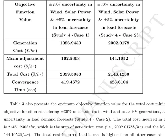
Generation Cost ($/hr) 1973.0461 Mean adjustment cost ($/hr) 41.7783
Total Cost ($/hr) 2014.8244 Convergence Time (sec) 306.1037
5.1.4 Study 4: Optimizing total cost minimization objective considering uncer-
17
tainties in wind, solar PV power generations, and load demand forecasts
18
In this Study, the total cost minimization objective function is optimized considering the un-
19
certainties in wind, solar PV powers and load demand forecasts. Table 3 shows the optimum
20
objective function value for the total cost minimization objective considering±20% uncertain-
21
ties in wind and solar PV power generations, and ±5% uncertainty in load demand forecast
22
(i.e., Study 4 - Case 1). Figure 3 shows the optimum generation schedules for Study 4. In
23
this Study 4 - Case 1, the amount of power scheduled from the wind farm is 34.6581MW and
24
the scheduled power from the solar PV system is 22.5471MW, which is the sum of solar PV
25
plant (i.e., 18.6659MW) and the aggregated battery (3.8812MW). The generation (i.e., ther-
26
mal, wind and solar PV) cost incurred in this case is 1996.9450$/hr, and the MAC obtained is
27