Jianguo Sun Xingqiu Zhao

Chapter 1 contains introductory material and examines basic concepts and point process models commonly used for analyzing panel count data. Specifically, chapter 3 deals with one-sample analysis of panel count data with a focus on nonparametric estimation of the mean function of the underlying recurring event process of interest.

Event History Studies

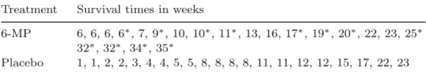
Failure Time Data on Remission Times of Acute
Recurrent Event Data on Times to Mammary Tumors 4
Reliability Study of Nuclear Plants
National Cooperative Gallstone Study
Bladder Cancer Study
Skin Cancer Chemoprevention Trial

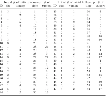
Table 1.4 provides a panel count data set for patients in the placebo arm of the bladder cancer study conducted by the Veterans Administration Co-. They are the size of the largest initial tumor and the number of initial tumors.

Table 1.1. Remission times in weeks for acute leukemia patients

Some Notation and Basic Concepts About

Counting Processes and Martingales
Some Commonly Used Models and Counting Processes 12
Nonparametric Estimation
Nonparametric Treatment Comparison
Regression Analysis Under the Cox Intensity Model

One is the estimator ˜Ak(t) obtained under the hypothesisH0 and the other is the estimator ˆAk(t) independent of the hypothesisH0. In the above model you could also allow Yi(t) and Zi(t) to depend on the type of recurring event.

Analysis of Panel Count Data

Some Features of Panel Count Data

Compared to failure time and recurring event data, panel count data have some similarities as well as some unique features. For the same reason, one usually focuses only on the average function of the underlying recurrent event process for the analysis of panel count data.

Outline

These include variable selection, analysis of mixed repeated-event and panel count data, and analysis of panel count data derived from multistate models. In addition, some discussions of Bayesian approaches to the analysis of panel count data and the analysis of panel count data derived from mixture models are also provided.

Introduction

Similar to the two methods discussed in Section 2.2 for count data, one is a probability-based method and the other is an estimating equation-based method.

Regression Analysis of Count Data

Likelihood-Based Procedures

It is easy to show that ˆβP is consistent and its distribution can be approximated by the normal distribution with mean β0, the true value of β, and the covariance matrix. Moreover, their joint distribution can be asymptotically approximated by the multivariate normal distribution with mean (βT0, γ0)T and covariance matrix defined by.

Estimating Equation-Based Procedures

In this case, assuming that we can treat {(Ni,Zi)}ni=1 as i.i.d., one can estimate V ar( ˆβP P) by the robust estimator.

Discussion

One can easily show that the estimator of β given by the solution of the equation above is consistent. Furthermore, one can approximate its distribution asymptotically by the normal distribution with meanβ0 and the covariance matrix.

Parametric Maximum Likelihood Estimation of Panel Count

Analysis Under Poisson Models
Analysis Under Mixed Poisson Models
An Illustration
Discussion

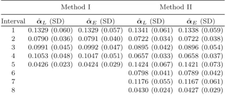
For convenience, it is assumed below that the observation is at the endpoint of each 10-week interval. Clearly, these general arguments apply to the analysis of the panel count data considered here.

Table 2.1. Observed number of k-tumored animals at interval i (a) Males (b) Females

Regression Analysis with Piecewise Models

Likelihood-Based Approach
Estimating Equation-Based Approach
An Illustration
Discussion

In this case, the robust estimator of the asymptotic covariance matrix ˆβE and ˆαE is given by . They are the number of initial tumors and the size of the largest initial tumor.

Table 2.2. Estimated covariate eﬀects for the bladder tumor data

Bibliography, Discussion, and Remarks

Regarding the comparison of the two estimation procedures discussed above, it is clear that the likelihood-based approach should be used if the mixed Poisson process assumption is reasonable. Of course, one can also question the appropriateness of another assumption behind both approaches, the piecewise model assumption for the baseline rate function.

Introduction

In Section 3.2, we first discuss some likelihood-based procedures for the nonparametric estimation of the mean function μ(t). One could also directly derive an estimator of the mean function based on the estimated degree function.

Likelihood-Based Estimation of the Mean Function

Non-homogeneous Poisson Process-Based Estimator

Then the log likelihood functionl(μ) can be rewritten as. 3.3) It is clear that only the values of μ(t) can be estimated at the sl's. As mentioned above, although the estimator ˆμF(t) is derived under the non-homogeneous Poisson process assumption, it is consistent and can be applied without the assumption.

Other Likelihood-Based Estimators

It is also easy to see that determining the NPMLE may not be computationally easy. Let Sl denote the set of indices of subjects observed in sl and define wl = |Sl|, the number of elements in Sl.

Isotonic Regression-Based Estimation of the Mean Function . 52

Illustrations

Assume that the feedwater flow loss numbers for all 30 nuclear plants follow the same counting process. Figure 3.1 presents the IRE of the average number of losses to feedwater flow given by the max-min formula.

Fig. 3.1. IRE of the average number of losses of feedwater ﬂow

Discussion

Regarding the asymptotic properties of NPMLE and IRE, Wellner and Zhang (2000) prove that under some regularity conditions, both estimators are stable in L2. An alternative is to first estimate the rate function μ(t) and then estimate μ(t) from the integral of the estimator of the rate function.

Generalized Isotonic Regression-Based Estimation of the

Generalized Isotonic Regression Estimators

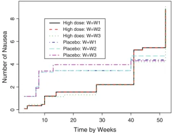
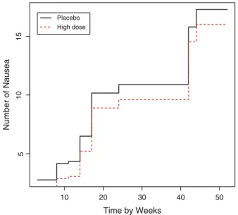
GIRE gives a class of estimators of the mean function μ(t) depending on the choice of weight matrix W and in theory any symmetric matrix can be used. In this case, LGI(μ|W) becomes a weighted least-squares function, and their well-known choice is to take w(sj, sj) to be the inverse of the variance of ni,j or its approximation.

Determination of the GIRE

It can also be shown that the kth step estimator μ(GIk) defined in (3.8) is the left derivative of the largest convex minor of the cumulative sum diagram. In the above, bjj(μ) is the element (j, j) of the matrix Bn(W) and therefore (μ) the j component of the vector.

An Illustration

On the other hand, it is easy to see that for a given subject observed atsj−1, the person may not be observed atsj. It is interesting to see that the estimators with different weighting matrices are similar for both groups.

Estimation of the Rate Function

Raw Estimators of the Rate Function
Smooth Estimators of the Rate Function
Illustrations
Discussion

Regarding the kernel estimators, it is clear that the value of the bandwidth h determines the smoothness of the estimator. Note that here, as above, IRE is used to determine the estimator of (3.12).

Fig. 3.5. Estimated loss rates of feedwater ﬂow

Bibliography, Discussion, and Remarks

Hu et al. (2009a) proposed a class of mean function estimators based on generalized isotonic regression, GIRE, using a weighted least squares criterion. Other authors who have considered nonparametric estimation of the mean or recurrence rate function based on the number of panels include Lu et al. (2007) and Hu et al. (2009b).

Introduction

Section 4.5 discusses this situation and presents a class of nonparametric testing procedures that allow different observation processes for the subjects in different treatment groups.

Two-Sample Comparison of Cumulative Mean Functions

Nonparametric Test Procedure I

That is, USF represents the integrated weighted difference between an individual treatment group estimator ˆμI,1(t) and the overall estimator ˆμI(t) of the common mean function of the Ni(t)'s under the null hypothesisH0. Note that this is often the case, for example, in clinical trials where randomization is used to assign subjects to different groups.

Nonparametric Test Procedure II

In this case, the Zis can be defined as the dose amounts given to the animals. It therefore follows, as above, that the test of the null hypothesis H0 can be carried out using the statistic UP SZ∗ = UP SZ/σˆP SZ, based on the standard normal distribution.

Discussion

As a result, the asymptotic distributions of the USF and UP SZ statistics, with the IRE replaced by the NPMLE, are still unknown. As an alternative to using the NPMLE of the mean function, Balakrishnan and Zhao(2010a) suggest using the statistic.

General p-Sample Comparison of Cumulative Mean Functions 77

NPMLE-Based Nonparametric Procedures

On the other hand, all the test statistics discussed above have similar meanings to some summation of differences between two estimators of the same function. For example, the NPMLE feature ˆμF(t), which plays a key role in the asymptotic normality of the functional ˆμF(t) and motivates the test statistic UBZ2,l is.

Discussion

It follows that the null hypothesis H0∗ can be tested using the statistic UBZ∗ 2 = UBZT 2ΣˆBZ−12UBZ2, based on the χ2 distribution with (p−1) degrees of freedom. As with UBZ1, the use of UBZ2 requires the selection of the weight processes Wn,l(t)'s and it is clear that the discussion about this in the previous subsection applies here.

Numerical Comparison and Illustration

Analysis of National Cooperative Gallstone Study
Numerical Comparison of the Test Procedures
Test Statistics
An Application
Discussion

For the statistics presented in the previous sections, the difference concerns the estimated average functions of the underlying repeated event processes given the observation processes. In other words, the difference does not include or use the information involved in the (assumed to be identical) observational processes.

Table 4.1. Test results for the ﬂoating gallstone data

Bibliography, Discussion, and Remarks

As discussed in Chapter 3 on nonparametric estimation from panel count data and in this chapter on testing procedures based on the NPMLE, one can easily see that the task would be very difficult or nearly impossible. It is worth noting that the way in which test statistics are developed here is actually the same as that used for the case of recurrent event data (Cook and Lawless, 2007) and also similar for the case of error time data (Kalbﬂeisch and Prentice, 2002) . ).

Introduction

Accordingly, Sections 5.3 and 5.4 present two types of equation estimation approaches, which neither depend on any distributional assumptions on N(t) nor require estimation of unknown functions. Accordingly, in section 5.5 we consider a class of semiparametric transformation models that include model (1.4) as a special case and also allow Z(t) to be time dependent.

Analysis by the Likelihood-Based Approach

A Semiparametric Maximum Pseudo-likelihood

It can be easily shown that the logarithm of the pseudo-likelihood function lp(μ,β) is a concave function of β for a given μ0(t) and its value increases after each iteration (Zhang,2002). Note that we assumed above that Ni(t) are inhomogeneous Poisson processes to derive the estimators ˆμP L(t) and ˆβP L .

A Semiparametric Spline-Based Maximum Likelihood

Let the ˆαls and ˆβSL denote the maximum likelihood estimators of the αls and β resulting from the maximization of lp(αls,β) given above. ThenLu et al.(2009) show that under some regularity conditions ˆμSL(t) and ˆβSL are consistent and ˆβSL asymptotically follows a normal distribution.

Discussion

In the next three sections, the estimating equation approach is used to derive estimators of the regression parameter β. It can be seen that the resulting estimation procedures are free from the estimation of unknown functions or additional parameters, and that the asymptotic properties of the resulting estimators can be determined relatively easily.

Analysis by the Estimating Equation Approach I

Assumptions and Models

We also assume that the average function of Ni(t) is given by model (1.4), as in the previous section. In the above model, ˜μ0(t) is a completely unspecified function, since μ0(t) and γ is a p-dimensional vector of regression parameters representing the effects of covariates on ˜Hi(t).

Estimation of All Regression Parameters

It can be easily shown that UI(β,γ,τ) asymptotically has expectation zero under the true values of the parameters (Sun and Wei For estimating τ one can use the partial likelihood-score function. Sun and Wei (2000) show that for large, the distribution of ˆβI − β0 can be approximated by a normal distribution with mean zero and the covariance matrix D(ˆθ)Γ(ˆθ)D(ˆθ).

Estimation with Same Follow-Up Times

Then it can be easily shown that for larger, the distributions of ˆγ −γ0 and ˆτ −τ0 can also be approximated by the normal distributions with mean zero and the covariance matrices. Furthermore, for large, one can approximate the distribution of ˆβI,1 −β0 by the normal distribution with mean zero and the covariance matrix.

Analysis by the Estimating Equation Approach II

A Conditional Estimating Equation Procedure

To motivate the new estimation function, note that the estimation function UI given in (5.7) is essentially constructed based on the summary statistic Ni(t)dHi(t). One can show that for any counting process that satisfies (5.10), the estimation function UIIC(β;w) given in (5.11) has mean zero.

An Unconditional Estimating Equation Procedure

Hu et al. (2003) show that the ˆβMII estimator is consistent and distributional.

Discussion

As in many cases, this is not a simple problem and it is also clear that the weight function does not necessarily have to be deterministic. In this case it is similar and simple to derive some estimators of β and determine their asymptotic properties, as above.

Analysis with Semiparametric Transformation Models

Assumptions and Models
Estimation Procedure
Determination of Estimators
A Goodness-of-Fit Test

Lin et al.(2001) examine, among others, model (5.15) for regression analysis of recurring event data. For determining ˆβT and ˆμ0(t) for a given data set, another issue is to choose or specify the function g in model (5.15).

Analysis of National Cooperative Gallstone Study

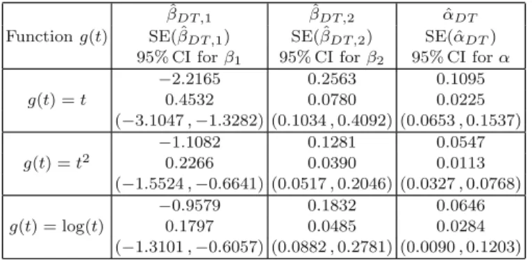
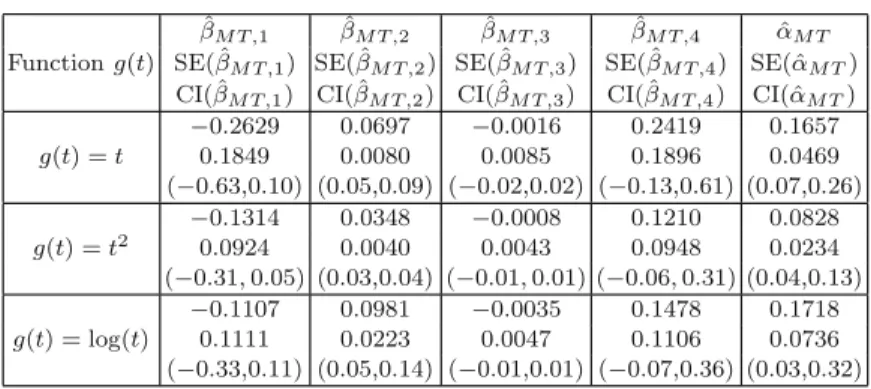
Now we consider the application of the estimation procedure derived based on the semiparametric transformation model (5.15). It is interesting to note that the semiparametric transformation model (5.15) with either g(t) = t or g(t) = log(t) seems to be a better or more appropriate choice than the one with g(t) = t2.

Fig. 5.1. Estimated mean functions of the occurrence processes of nausea under model (5.15) with g(t) = log(t)

Bibliography, Discussion, and Remarks

As for the comparison between Poisson or probability-based methods and estimation equation-based procedures, as mentioned earlier, the former could be much more complicated than the latter. On the other hand, it is clear that the former could be more efficient than the latter if the assumption related to the Poisson process holds.

Introduction

The new model is conditional and assumes that the rate of occurrence of repeated events of interest may depend on the observation process. For both cases, the implication is that recurrent events of interest may continue to occur after the follow-up time, albeit unobservable.

Analysis by a Joint Modeling Procedure

Assumptions and Models

In the presence of terminal events, an important problem arises when the terminal event is correlated with the recurring events of interest as well as with the observation process. Among the above models, it is easy to see that the relationship between the recurring events of interest process Ni(t) and the observation process ˜Hi(t) is represented by the regression parameterβ2.

Estimation of Parameters

To estimate θ it is natural to maximize L(θ) by replacing the onions with their predicted values given by (6.6). Note that it is possible to derive a consistent estimator of the covariance matrix of ˆβJ, but the estimator might be too complicated to be useful.

Discussion

In the case of time-dependent covariates, it is still possible to use model (6.2) and the estimation function given in (6.12), but different estimation procedures may be required relative to models (6.3) and (6.4). Given the evaluation function UJ(β) given in (6.12), as with the evaluation function given in (6.5), we could add some weights at the beginning of the integration.

Analysis by a Robust Estimation Procedure

Inference Procedure
Analysis of Bladder Cancer Study
Discussion

Note that the approach discussed in the previous section requires the assumption of the Poisson process for the observation process. To estimate the regression parameter β in the above model, an estimation function similar to UR(β1) given in (6.17) can be derived.

Fig. 6.1. The IRE for bladder tumor recurrence processes

Analysis with Semiparametric Transformation Models

An Illustration
Discussion

For example, one can take Q(Fit) = ˜Hi(t−) if one believes that Ni(t) may depend on the total number of observations ahead of time. We assume that the visit or observation process and the recurrence process of the bladder tumors follow the models (5.16) and (6.18), respectively.

Table 6.1. Estimated regression parameters with Q(F it ) = ˜ H i (t−)

Analysis with Dependent Terminal Events

Estimation of Regression Parameters
Reanalysis of Bladder Cancer Study
Discussion

Similarly, the effect of the visit or observation process on the terminal event also represents the adjusted recurring event process. Instead of model (6.20), one can directly model the marginal mean function of the unadjusted recurring event process of interest.

Bibliography, Discussion, and Remarks

On the other hand, many authors have investigated the situation where there is a terminal event, such as a survival event related to the longitudinal process of interest. Sometimes it may be more natural to ask or model how the observation process depends on the history information of the repeated event process.

Introduction

More precisely, we consider the situation where the marginal average functions of each individual process of the repeated event we are interested in and the observation process can be characterized by the models (6.14) and (6.15), respectively. Finally, Section 7.6 provides some bibliographic notes and discusses some issues not touched upon in the previous sections.

Nonparametric Comparison of Cumulative Mean Functions

Two-Sample Nonparametric Test Procedures

The approach given below can be easily generalized to the situation where the observation times for different types of recurring events are different. It is clear that ifK = 1,UZV S reduces to the test statistic UP SZ discussed in Section.4.2.2 for univariate panel count data.

An Application

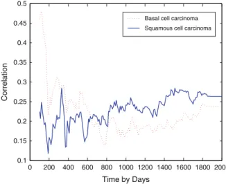
Estimated Mean Recurrence Functions of New Skin Cancers To apply the testing procedure discussed in the previous subsection, for subject i, define Ni1(t) and Ni2(t) as the processes representing the cumulative numbers of skin carcinoma occurrences basal cells and squamous cell carcinoma, respectively, until time t, i = 1,. Let μ11(t) and μ21(t) represent the mean cumulative incidence functions of basal cell carcinoma and squamous cell carcinoma, respectively, for patients in the DFMO treatment group.

Discussion

To be precise, let μkl(t) denote the mean function of the recurring event process for the kth recurring event of the type corresponding to treatment l,l = 1,. As already mentioned, of course the distributions of the observation times cannot be completely different between the treatment groups, otherwise a non-parametric comparison may not be possible.

Regression Analysis with Independent Observation Processes . 161

Estimation Procedure

Suppose the boundaries of S(kd)(t;γ) and Ek(t;γ) exist. Cai and Schaubel (2004) propose to estimate γ using the following estimation equation. Note that the last quantity ˆμ˜k(t;γ) is a generalization of the estimator (1.10) for the baseline mean function ˜μk(t) givenγ,i = 1,.

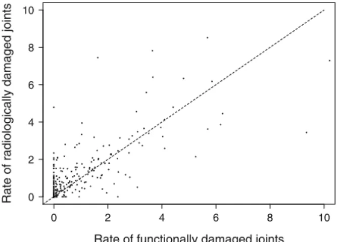
Analysis of Psoriatic Arthritis Data

Estimated effects of covariates on the assessment time processes and the processes of occurrence of the two types of damaged joints. The above multivariate analysis results indicate that all three basic covariates had significant effects on the frequency of occurrence of the two types of damaged joints.

Fig. 7.2. Empirical rate functions of two types of damaged joints

Discussion

Radiologically damaged joints − Univariate Radiologically damaged joints − Multivariable Functionally damaged joints − Univariate Functionally damaged joints − Multivariable. Estimated baseline mean functions for two types of damaged joints another indication that the former should be preferred over the latter in such situations.

Joint Regression Analysis with Dependent Observation

Analysis of Skin Cancer Chemoprevention Trial
Discussion

Incidence The frequency also does not seem to be significantly related to the patient's age and gender. But the incidence rate appears to be positively related to the number of previous skin cancers.

Fig. 7.4. Estimated pointwise correlations between the cancer occurrence process and the observation process for two types of skin cancers

Conditional Regression Analysis with Dependent

Estimation Procedure
Determination of Estimators
Reanalysis of Skin Cancer Chemoprevention Trial
Discussion

The former Q assumes that the incidence of skin cancer may depend on the total number of patient visits. More specifically, all results indicate that the DFMO treatment did not appear to have a significant effect on the incidence of the two types of skin cancer.