An Introduction to the Design and Behavior of Bolted Joints: Second Edition, Revised and Expanded, John H. An Introduction to the Design and Behavior of Bolted Joints: Third Edition, Revised and Expanded, John H.
GOVERNING EQUATIONS
STATISTICAL AND CONTINUUM METHODS
The continuum approach requires that the mean free path of the molecules be very small compared to the smallest physical length scale of the £ow field (such as the diameter of a cylinder or other body around which the £uid is). . Other old variables can be defined in terms of molecular properties in an analogous way.
EULERIAN AND LAGRANGIAN COORDINATES
Then in the Lagrangian framework we follow this colored portion as it £overs and changes its shape, but we always consider the same particles of £uid. The independent variables in the Lagrangian system are x0, y0, z0, andt, where x0, y0, andz0 are the coordinates through which a specified $uid element passed at time 0.
MATERIAL DERIVATIVE
The left-hand side of this expression represents the total change in a as observed in the Lagrangian frame during timedt, and in the limit it represents the time derivative of a in the Lagrangian system, which will be denoted by Da=. It represents the total change in quantity as seen by an observer following. uid and sees a certain mass of £uid. The entire right-hand side of Eq. 1.1) represents the total change not expressed in Eulerian coordinates.
CONTROL VOLUMES
REYNOLDS’ TRANSPORT THEOREM
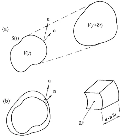
The combination of the arbitrary control volume and the Lagrangian coordinate system means that material derivatives of the volume integrals will be encountered. FIGURE 1.2 (a) Arbitrarily shaped control volume at times t and tþdt, and (b) superposition of control volumes at these times showing a dV element of the volume change.
CONSERVATION OF MASS
Equation (1.2) relates the lagrangian derivative of a volume integral of a given mass to a volume integral in which the integrand has only Eulerian derivatives. This equation can be converted to a volume integral in which the integrand contains only Eulerian derivatives by using Reynolds' transport theorem [Eq. 1.2)], where the £uid property is, in this case, the mass density.
CONSERVATION OF MOMENTUM
In this notation, a certain component of the voltage can be represented by the quantity sij, where the first subscript indicates that this voltage component acts. The left side of Eq. 1.4) represents the rate of change of momentum of a unit volume of the µuid (or the inertial force per unit volume).
CONSERVATION OF ENERGY
The work done on the fluid by these forces is given by the product of the velocity and the component of each force that is collinear with the velocity. Similarly, the second term on the left-hand side of the basic equation can be expanded by considering reuk to be the product of (e)(ruk) and 12rujujuk to be the product of ð12ujujÞðrukÞ.
DISCUSSION OF CONSERVATION EQUATIONS
The terms dropped in the final simplification were the mechanical energy terms. The first of these terms represents the conversion of mechanical energy into thermal energy due to the action of surface tension.
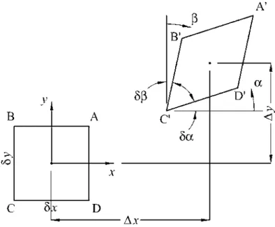
ROTATION AND RATE OF SHEAR
Thus the rate of clockwise rotation of the £uid element about its center of gravity is given by. If the analysis is carried out in the other planes, it can be verified that the rotation rate of the element about its own axes and the displacement rate are given by .
CONSTITUTIVE EQUATIONS
There are nine elements in the shear stress tensor, and each of these elements can be expressed as a linear combination of the nine elements in the strain-rate tensor, just as a vector can be represented as a linear combination of components of the basis vectors). Thus, in order for condition 3 to be satisfied, the coefficients of this part of the strain rate tensor must be zero.
VISCOSITY COEFFICIENTS
This average normal stress is the mechanical stress in the £uid and it is equal to one third of the trace of the stress tensor. That is, the difference between the thermodynamic pressure and the mechanical pressure is proportional to the divergence of the velocity vector.
NAVIER-STOKES EQUATIONS
For example, during the passage through a shock wave, the vibrational modes of energy are excited at the expense of the translational modes, so the bulk viscosity in this case will not be zero. In most common situations, it can be assumed that the fluid is incompressible and the dynamic viscosity is constant.
ENERGY EQUATION
Using the fact that in the ¢rst two terms of the stress tensor¼j for non-zero elements, this expression becomes. Using this result and the constitutive relation for heat £ux [Eq. 1.8)] in the energy conservation equation, Eq. 1.5), gives the energy equation for the Newtonian £uid.
GOVERNING EQUATIONS FOR NEWTONIAN FLUIDS
More often, however, thermal effects are unimportant and the continuity and Navier-Stokes equations alone must be solved. If the £uid is at rest, the velocity components will all be zero, so that the Navier-Stokes equations become (1.9a).
BOUNDARY CONDITIONS
The resulting equation must be expressed in terms of the Cartesian coordinates (x,y,z,t), the Cartesian velocity components (u,v,w) and the fluid density. The resulting equation must be expressed in terms of the cylindrical coordinates (R, y, z, t), the cylindrical velocity components ðuR;uy;uzÞ and the fluid density.
FLOW LINES
That is, the equation of the dashed line through the point ðx0;y0;z0Þ is obtained by Eq. Eliminating from these parametric equations, it appears that the equation of the dashed line passing through the point (1, 1) is at time t¼0.
CIRCULATION AND VORTICITY
These are the parametric equations of the dashed line passing through the point (1, 1), and they are valid for all times. That is, the vorticity is equal to twice the anti-symmetric part of the strain-rate tensor.
STREAM TUBES AND VORTEX TUBES
By analogy with streamlines and streamlines, the useful concepts of vortex lines and vortex tubes can be introduced. A vortex tube, the surface of which is infinitely small, is usually called an vortex ¢lament.
KINEMATICS OF VORTEX LINES
The cross-sectional area and shape at any other section of the vortex tube will generally be different. That is, the circulation around the limiting contour of the area A1 is equal to that around A2.
KELVIN’S THEOREM
Suppose that the pressure p can be considered as a function of the density, only as, for example, with isentropic flows. Recall that the right side of Eq. 3.1) could be proven to be zero by considering the fluid to be non-viscous, the body forces being conservative and the density constant, or the pressure being a function of the density alone.
BERNOULLI EQUATION
It should be remembered that it is valid for the steady £ow of a £uid in which viscous effects are negligible and in which any body force is conservative. 2=f·=fG¼FðtÞ ð3:2cÞ where FðtÞ is a function of time that can be added after integration over spatial coordinates. 3.2c) is valid for the irrotational motion of a £uid in which viscous fluxes are negligible and in which any body force is conservative.
CROCCO’S EQUATION
To determine the Croce equation, consider the flow of an inviscid material. uid in which there are no physical forces. Equation (3.3b) applies to a steady, adiabatic flow of an incompressible fluid in which there are no body forces.
VORTICITY EQUATION
For two-dimensional flows, the vorticity vector v will be perpendicular to the plane of the flow, so ðv·=Þu will be zero. Using the definition of enthalpy, show that the equivalent form of this equation.
IDEAL-FLUID FLOW
STREAM FUNCTION
FIGURE 4.1 Two streamlines showing the components of the volumetric flow rate over an element of the control surface connecting the streamlines. This property of the streamlines and equipotential lines is the basis of a numerical procedure for solving two-dimensional potential £ow problems.
COMPLEX POTENTIAL AND COMPLEX VELOCITY
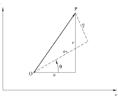
An expression for the complex velocity can be easily obtained in cylindrical coordinates by converting the Cartesian components of the velocity vector ðu; vÞto cylindrical componentsðuR;uyÞ. Based on this, each of the Cartesian velocity components can be expressed in terms of the two cylindrical components as follows:
UNIFORM FLOWS
Then the complex potential for such a £ow whose velocity magnitude is V will be in the positive direction.
SOURCE, SINK, AND VORTEX FLOWS
It is clear that the complex potential for a sink, which is a negative source, is obtained by substituting Eq. Then nc can be replaced by G=2p, giving the following complex potential for a positive (counterclockwise) vortex of strength G.
FLOW IN A SECTOR
Between these two lines, the streamlines are bounded by Rnsinny¼constant. This gives the £ow field shown in fig. From the foregoing, the complex potential for £ow in a corner or sector of anglep=nis. 4.10) gives the complex potential for a uniform straight line.
FLOW AROUND A SHARP EDGE
An important feature of this result is that the angle itself is a singular point at which the velocity components become infinite. Since also Randuyvary as the inverse of R1=2, it follows that the velocity is singular as the square root of the distance from the edge.
FLOW DUE TO A DOUBLET
However, it turns out that the doublet can be thought of as the merging of a source and a sink, and the required complex potential can be obtained by a limiting procedure that uses this fact. This interpretation leads to a better physical understanding of the doublet, and for this reason it will be followed here before studying the £ow ¢eld. Although the direction of the £ow along the streamlines can be deduced from the source and sink interpretation, this will be checked by evaluating the velocity components.
CIRCULAR CYLINDER WITHOUT CIRCULATION
The £ow field due to the doublet encounters that due to the uniform £ow and is bent downstream. Similarly, the drag force acting on the cylinder is zero due to the symmetry of the £ode around the axis.
CIRCULAR CYLINDER WITH CIRCULATION
It is clear that if the circulation is increased above this value, the single stagnation point cannot remain on the surface of the cylinder. Since it seems likely that any stagnation points there may not lie on the surface of the will.
BLASIUS’ INTEGRAL LAWS
The last equality follows by comparing the extended form of the complex integral with the expressions derived above for the body forces X and Y. That is, the complex force XiY can be evaluated. The last equality follows from an equation of the real part of the complex integral with the expression derived for M.
FORCE AND MOMENT ON A CIRCULAR CYLINDER
But inspection of the derived expression for W2ðzÞ above shows that the only singularity is atz¼0, which corresponds to the doublet and the vortex located there. Moreover, W2ðzÞ is in its Laurent series form about z¼0, from which it is seen that the only term of the form1=zis is the fourth.
CONFORMAL TRANSFORMATIONS
That is, Laplace's equation in the z-plane transforms to Laplace's equation in the z-plane, provided that these two planes are related by a conformal transformation. Then, since both and two must satisfy Laplace's equation, it follows that a complex potential in the plane is also a valid complex potential in the plane, and vice versa.
JOUKOWSKI TRANSFORMATION
This last result shows that if a smooth curve passes through the point z¼c, the corresponding curve in the z plane will form a cutting edge or tip. This means that if a smooth curve passes through any of the critical points z¼ c, the corresponding curve in the z plane will contain a blade at the corresponding critical point z=2c.
FLOW AROUND ELLIPSES
Then, to obtain the complex potential for a uniform islet of size approaching this ellipse at an angle of attack, the same islet should be considered to approach the circular cylinder in the z-plane. The stagnation points in the z-plane are located at z¼aeia and z¼aeiðaþpÞ, that is, atz¼ aeia. 4.20), are the corresponding points in the z-plane.
KUTTA CONDITION AND THE FLAT-PLATE AIRFOIL
In the actual flow configuration, the fluid would separate at the leading edge and reattach to the upper side of the airfoil. Then, if we denote the lift force by Y and use the circulation value given by Eq.
SYMMETRICAL JOUKOWSKI AIRFOIL
To determine the maximum thickness t, the equation of the airfoil surface must be obtained. So points on the surface of the airfoil will be defined by z¼c½1þeð1cosnÞeinþ cein 1þeð1cosnÞ.
CIRCULAR-ARC AIRFOIL
This is the equation of the aerodynamic surface in the Z plane, but still includes the variables. Then the equation of the in-plane aerodynamic surface can be written in the form.
JOUKOWSKI AIRFOIL
Despite this local inaccuracy, the results derived above are representative of the £ow around thin curved airfoils. These results follow from the observation that cosdreplacesmas are used in the symmetric Joukowski airfoil and msindreplacesmas used in the circular arc airfoil.
SCHWARZ-CHRISTOFFEL TRANSFORMATION
To find the magnitude of the uniform velocity, it is observed from the mapping function that if z. Substitution of b¼a in the complex potential confirms the result obtained above using the Schwarz-Christo¡el transformation.
SOURCE IN A CHANNEL
This result can be checked by using the result for the uniform £ow of magnitudeU past an ellipse of major semi-axis ðaþb2=aÞ and minor semi-axis ðab2=aÞ, the latter being along the axis. The resulting complex potential is given by Eq. 4.21b), which was obtained using the Joukowski transformation. Equation (4.26) is the complex potential for the £ow con¢gurations shown in fig. Figure 4.20b shows the £ow¢eld due to a source located on the centerline of an infinitely long channel or at the center of the end of a semi-in¢nite channel.
FLOW THROUGH AN APERTURE
Then along the free streamlines, z¼eiy, which is the equation of the unit circle in the zplane. To evaluate the contraction coe⁄cientCc, the equation for the free streamline B0C0 will be established.
FLOW PAST A VERTICAL FLAT PLATE
So obtain the complex potential for the flow around a right-angled bend in terms of the channel width and the approach velocity U. Noting that the strength of the source in the z-plane ism¼2UH, obtain the complex potential for the flow field in the z-plane.

VELOCITY POTENTIAL
For asymmetric £currents there will be no variation in the £uid properties from 0 to 2p while holding randya constant. dimensionality of the current field. Then the equation to be satisfied by the velocity potential is Laplace's equation given by Eq. Thus, by extending the Laplace in spherical coordinates and using the fact that @=@o¼0 for asymmetric currents, the equation must be satisfied.
STOKES’ STREAM FUNCTION
First, the statement will be assumed to be true and to constitute the definition of a quantity. It will then be shown that as a result of this definition the velocity components must be related to this function by Eqs.
SOLUTION OF THE POTENTIAL EQUATION
Therefore, if either roryal is changed, one side of the equation will change while the other will not. This is a one-dimensional equation, and its solution will therefore have the form RðrÞ ¼Kra.
UNIFORM FLOW
In light of the nature of this function, it is often referred to as Legendre's polynomial of order l. Both of the methods outlined above for evaluating the stream function are useful, and each will be used in the following sections. The specific method used will depend on the complexity of the problem, and it is clear that the second method is convenient only for Very simple.
SOURCE AND SINK
Here the sourceQ will be considered to be slightly to the right of O, so that the amount £uid the surface generated by OP will be 2pcþQ. It now becomes clear that if the source Q was considered to be slightly to the left of the origin, the constant term in Eq.
FLOW DUE TO A DOUBLET
Equation (5.7a) is the velocity potential for a positive doublet of strengthm, that is, a doublet that emits £uid along the negative part of the reference axis and absorbs £uid along the positive part. Equation (5.7b) gives the stream function for a doublet that discharges £uid along the negative part of the reference axis and attracts £uid along the positive part of the reference axis.
FLOW NEAR A BLUNT NOSE
Then the shell could be adapted to the shape of the surface corresponding to toc=0 and the source could be removed without disturbing the external flow. Equations (5.8) can be used to derive the velocity and pressure distributions near the nose of a blunt axisymmetric body such as an aircraft fuselage or a submarine hull.
FLOW AROUND A SPHERE
The £uid emanating from the source located at the origin does not mix with the £uid constituting the uniform £ow. Then, choosing m¼2pUa3, the current functions for a uniform £ow of magnitudeU approaching a sphere of radiusais.
LINE-DISTRIBUTED SOURCE
5.7, it will be noted that the cylindrical radius R¼rsiny¼Zsina remains constant throughout the integration. Using these relations, the expression for the stream function for a line source of unit length qper and length Lis.
SPHERE IN THE FLOW FIELD OF A SOURCE
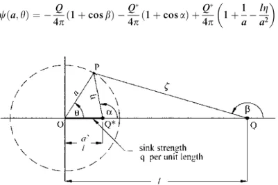
FIGURE 5.8 Superposition of a line sink with powerq per unit length, a source of powerQ, and a source of powerQ near a sphere of radius. Using the fact that Q¼aQ=earthq¼lQ=a2¼Q=a, we obtain an expression for the velocity potential for a sphere of radius Q in the presence of a power source.
RANKINE SOLIDS