No part of this publication may be reproduced, stored in a retrieval system, or transmitted in any form or by any means, electronic, mechanical, photocopying, recording, scanning or otherwise, except under the terms of the Copyright, Designs and Patents Act of in 1988 or under the terms of a license issued by Copyright Licensing Agency Ltd, 90 Tottenham Court Road, London W1T 4LP, UK, without the written permission of the publisher. It is sold on the condition that the Publisher does not engage in the provision of professional services.
Discrete and Continuous Markov Processes 71
List of Tables
List of Illustrations
Preface
INTENDED AUDIENCE
The detailed step-by-step derivation of queue results makes it an excellent text for academic courses, as well as a text for self-study.
ORGANISATION OF THIS BOOK
ACKNOWLEDGEMENTS
Preliminaries
PROBABILITY THEORY
- Sample Spaces and Axioms of Probability
- Conditional Probability and Independence
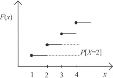
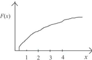
- Random Variables and Distributions
- Expected Values and Variances
- Joint Random Variables and Their Distributions
- Independence of Random Variables
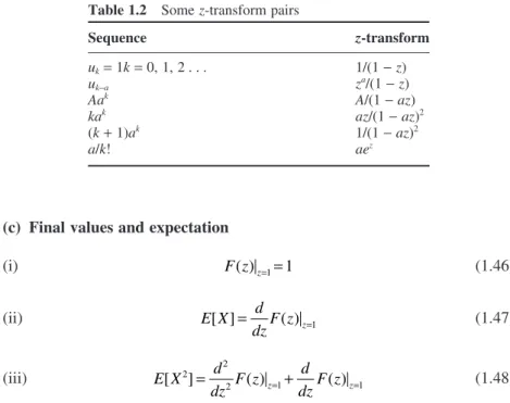
- Properties of z-Transforms
A continuous random variable X is an exponential random variable with parameter l > 0 if its density function is defined by. Find the expected value of a Cauchy random variable X, where the density function is defined as.
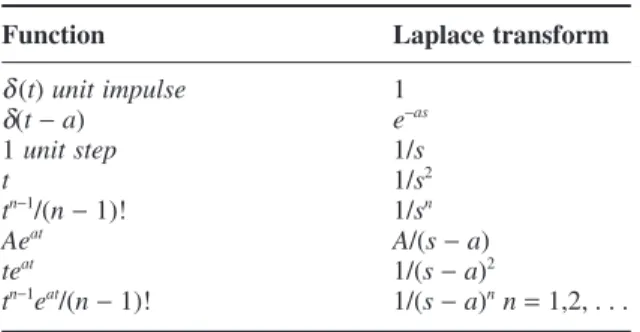
LAPLACE TRANSFORMS
- Properties of the Laplace Transform
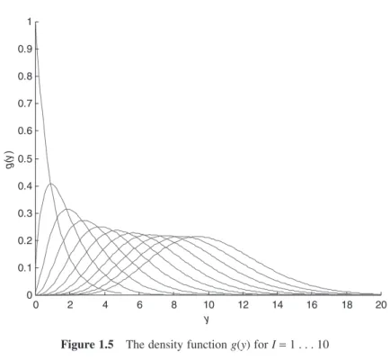
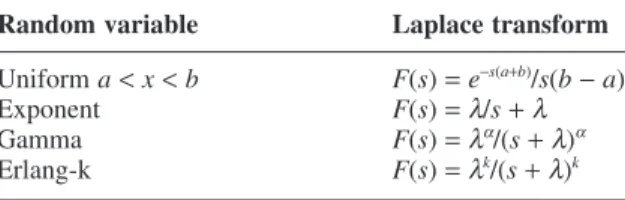
The Laplace transform enjoys many of the same properties as the z-transform as applied to probability theory. Derive the Laplace transforms for the exponential and k-stage Erlang probability density functions, then calculate their means and variances.
MATRIX OPERATIONS
- Matrix Basics
- Eigenvalues, Eigenvectors and Spectral Representation
- Matrix Calculus
We summarize some of the properties of matrices that are useful in their manipulation. Here, we summarize some of the properties of eigenvalues and eigenvectors: i) The sum of the eigenvalues of à is equal to the sum of the diagonal entries of Ã. The sum of the diagonal entries of à is called the trace of Ã. l kn are eigenvectors of Ãk, and we have
Problems
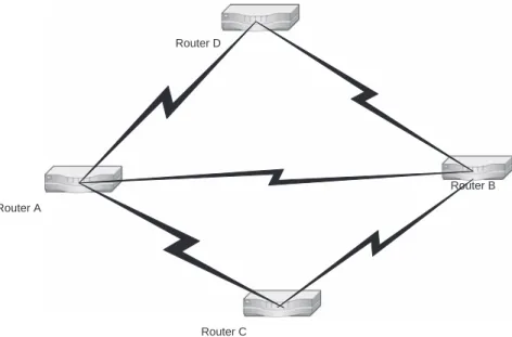
Using the value of the determined parameter a, calculate the time t0 such that the probability that T is smaller than t0 is 0.05. What is the probability that a message can be sent from router A to router B (assume packets are moving in the direction of the destination).
Introduction to Queueing Systems
NOMENCLATURE OF A QUEUEING SYSTEM
- Characteristics of the Input Process
- Characteristics of the System Structure
- Characteristics of the Output Process
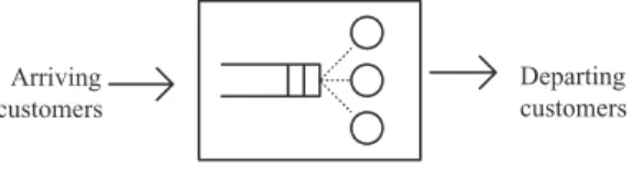
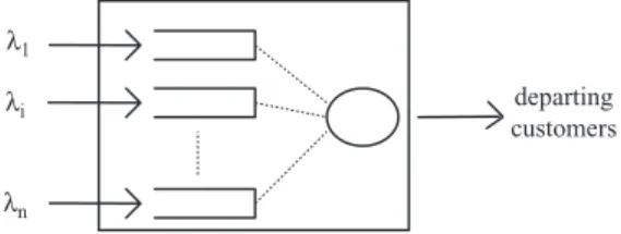
On the other hand, the analysis of a finite-size customer population queuing system is more complicated because the arrival process is affected by the number of customers already in the system. When customers arrive regularly at a certain interval, the arrival pattern is easily described by a single number - the arrival rate. In a multi-server queuing system, as shown in Figure 2.2 (a), the system capacity is the sum of the maximum queue size and the number of servers.
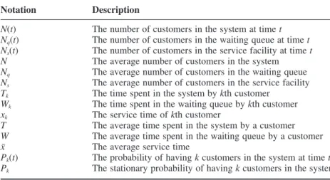
RANDOM VARIABLES AND THEIR RELATIONSHIPS
Wk The time kth customer spent in the queue. xk The service time of kth customer. T The average time a customer spends in the system. W The average time a customer spends in queue x¯ The average service time. Pk(t) The probability that there are k customers in the system at time t Pk The stationary probability that there are k customers in the system RANDOM VARIABLES AND THEIR RELATIONS 49.
KENDALL NOTATION
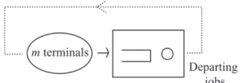
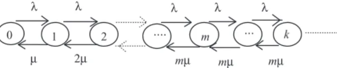
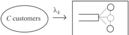
There are two ways to model this terminal-CPU system. i) First, we assume that the think times (or job submission times) and CPU processing times are exponentially distributed, so the arrival process is Poisson. Therefore, the system can be modeled as an M/M/1/m system, as shown in Figure 2.4, with arrival rate l(k) given by expression (2.10) above. This model is commonly known as a 'finite population' queuing model or 'machine repairman' model in classical queuing theory. ii) An alternative way is to model the system as a closed queuing network of two queues, as shown in Figure 2.5; one for the terminal and the other for the CPU.
LITTLE’S THEOREM
- General Applications of Little’s Theorem
- Ergodicity
Here, the time spent in the system (Tsub) is the total time required to traverse the switch and the transmission line B. TB is the time a packet spends being transmitted over Line B. Nsw is the number of packets at the switch. NB is the number of packets at line B. lB is the arrival rate of packets to line B.

RESOURCE UTILIZATION AND TRAFFIC INTENSITY
To better understand the physical meaning of this entity, take a look at the traffic presented to a single resource. One erlang of traffic corresponds to a single user using that resource 100% of the time or alternatively 10 users each occupying the resource 10% of the time. A traffic intensity greater than one indicates that customers are arriving faster than they are being served and is a good indication of the minimum number of servers required to achieve a stable system.
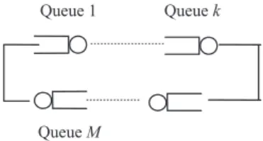
FLOW CONSERVATION LAW
Consider the queuing system shown below where we have customers arriving at Queue 1 and Queue 2 with rates ga and gb respectively. If the branching probability p in Queue 2 is 0.5, calculate the effective arrival rates in both queues. Denote the effective arrival rates at Queue 1 and Queue 2 as l1 and l2, respectively, then we have the following expressions under the flow conservation principle:.
POISSON PROCESS
- The Poisson Process – A Limiting Case
- The Poisson Process – An Arrival Perspective
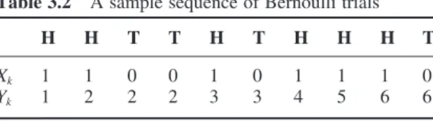
Therefore, the Poisson process can be considered as the superposition of a large number of Bernoulli arrival processes. If this counting process satisfies the following assumptions, it is a Poisson process. i) The distribution of the number of arrivals in a time interval depends only on the length of this interval. This property is known as independent increments. ii) The number of arrivals in non-overlapping intervals is statistically independent.
PROPERTIES OF THE POISSON PROCESS .1 Superposition Property
- Decomposition Property
- Exponentially Distributed Inter-arrival Times
- Memoryless (Markovian) Property of Inter-arrival Times
- Poisson Arrivals During a Random Time Interval
The decay property is just the reverse of the previous property, as shown in Figure 2.12, where a Poisson process. If we assume that I is distributed with a probability density function A(t) and I is independent of the Poisson process, then. What is the average number of cars within the premises of the inspection center (including the cafeteria).

Discrete and Continuous Markov Processes
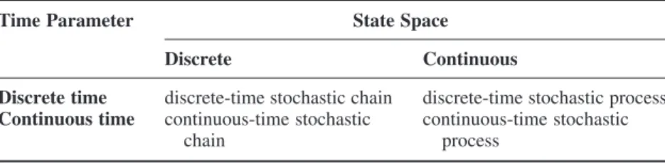
STOCHASTIC PROCESSES
In the stock counter example, the state space is the set of all prices of that particular counter throughout the day. For example, the set of positive integers {n} in the interval [a, b] is infinite or countably infinite, while the set of real numbers in the same interval [a, b] is infinite. The statistical dependence of a stochastic process refers to the relationship between a random variable and others in the same family.
DISCRETE-TIME MARKOV CHAINS
- Defi nition of Discrete-time Markov Chains
- Matrix Formulation of State Probabilities
- General Transient Solutions for State Probabilities
- Steady-state Behaviour of a Markov Chain
- Reducibility and Periodicity of a Markov Chain
- Sojourn Times of a Discrete-time Markov Chain
The conditional probability on the right-hand side of equation (3.3) is the probability that the chain goes from state i at time step k to state j at time step k + 1 – the so-called (one-step) transition probability. The conditional probability shown in equation (3.3) only expresses the dynamics (or movement) of the chain. The previous residence time result is in line with the memoryless property of a Markov chain.
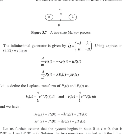
CONTINUOUS-TIME MARKOV CHAINS
- Defi nition of Continuous-time Markov Chains
- Sojourn Times of a Continuous-time Markov Chains
- State Probability Distribution
- Comparison of Transition-rate and Transition-probability Matrices
The exponential distribution is a continuous version that also has this property, and we will show later that the residence times of a Markov chain with a continuous time are exponentially distributed. Similar to a discrete-time Markov chain, the residence time of a continuous-time Markov chain is the time the chain spends in a particular state. We will show that the residence times of a continuous-time Markov chain are indeed exponentially distributed using the above definition.
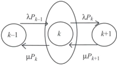
BIRTH-DEATH PROCESSES
A process of pure death is one in which members of the population only die, but none are born. Outward immigration is assumed to contribute to an exponential growth rate q of the population. Assume that births are independent of deaths as well as of outward immigration.
Single-Queue Markovian Systems
CLASSICAL M/M/1 QUEUE
- Global and Local Balance Concepts
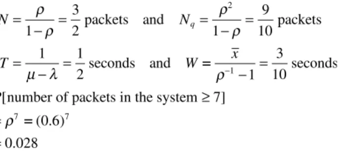
- Performance Measures of the M/M/1 System
The arrival rate l and the service rate m do not depend on the number of customers in the system, so they are state independent. Let us first focus our attention on the number of customers N(t) in the system at time t. We see that the probability of having k customers in the system is a geometric random variable with parameter r.
PASTA – POISSON ARRIVALS SEE TIME AVERAGES
It should be noted that these steady-state performance measurements are derived without any assumptions about the queue discipline, and they apply to all queue disciplines that are in storage of work. Simply put, job retention means that the server is always busy as long as there are clients on the system. However, we know that the event of an arrival at time t is independent of the process {N(t) = k} due to the memoryless properties of the Poisson process.
M/M/1 SYSTEM TIME (DELAY) DISTRIBUTION
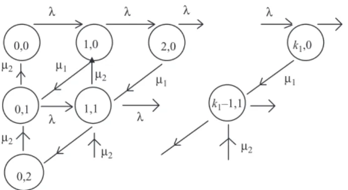
Assuming that the clinic is large enough to accommodate a large number of patients, the situation can be modeled as an M/M/1 queue. Voice packets are always accepted into the transmission buffer, and data packets are only accepted if the total number of packets in the system is less than N. The time required to process each task is exponentially distributed with mean 1/m, regardless of the number jobs in the system. i) Draw the state transition diagram of this system and write the global and local balance equation. ii) Find the steady state probability Pk that there are k jobs on the computer and then find the average number of jobs. iii).
M/M/1/S QUEUEING SYSTEMS
- Blocking Probability
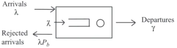
- Performance Measures of M/M/1/S Systems
This result is intuitively correct, as it shows that the blocking probability is the probability when the system is saturated. For r = 1, the expression for the blocking probability must be evaluated using L'Hopital's rule, and we have it. ii) The average number of customers in the system is given by. Since customers are blocked when they are in the customer S system, the actual arrival rate of customers admitted to the system is the same.
MULTI-SERVER SYSTEMS – M/M/m
- Performance Measures of M/M/m Systems
- Waiting Time Distribution of M/M/m
This situation occurs when there are more than m clients in the system, so we have He/she can find k customers waiting in the queue upon arrival, which means there are n = (k + m) customers in the system. His/her waiting time is simply the sum of the service time xj (j = 1, . . . k) of those k customers in the queue as well as the service time x of those customers currently in service.
ERLANG’S LOSS QUEUEING SYSTEMS – M/M/m/m SYSTEMS
- Performance Measures of the M/M/m/m
This system is also stable, even for r = l/mm ≥ 1, due to this self-regulating mechanism whereby customers are turned away when the system is full. i). This probability is the block probability and is equal to the probability that the system is full. Because there is no waiting time, the system time (or delay) is the same as the service time and has the same distribution:
ENGSET’S LOSS SYSTEMS
- Performance Measures of M/M/m/m with Finite Customer Population
If the population size C of the arriving customers is the same as the number of servers in the system, i.e. If the population size C of the arriving customers is the same as the number of servers in the system, i.e.
CONSIDERATIONS FOR APPLICATIONS OF QUEUEING MODELS
Draw the state transition diagram and show that the empty system probability is (1 + r)−S. Employees are expected to collectively generate Poisson outbound calls at a rate of 30 calls per minute. If another doctor is employed to care for the patients, find the average number of patients in the dispensary, assuming that the rate of arrival and service have remained the same as before.
Semi-Markovian Queueing Systems
THE M/G/1 QUEUEING SYSTEM
- The Imbedded Markov-Chain Approach
- Analysis of M/G/1 Queue Using Imbedded Markov-Chain Approach
- Distribution of System State
- Distribution of System Time
We assume that the mean E(x) and the second moment E(x2) of the service time distribution exist and are finite. We also assume that the service times are independent of the arrival process as well as the number of customers in the system. After obtaining the excitation function of the system state in Equation (5.16), we can proceed to find the average value N as.
THE RESIDUAL SERVICE TIME APPROACH
- Performance Measures of M/G/1
Here we assume that the service time distribution is independent of the state of the system; this is the number of clients in the system. It is interesting to note that the waiting time is a function of both the mean and the second moment of the service time. This is analogous to the situation in Figure 5.2, and the time a passenger needs to wait for the train to arrive is actually the remaining service time seen by an arriving customer to a non-empty system.

M/G/1 WITH SERVICE VOCATIONS
- Performance Measures of M/G/1 with Service Vacations
Here, we denote Rs as the average remaining service time and Rv as the average remaining vacation time. The busy periods between those holiday periods are not shown in the diagram because they are taken care of by the remaining service time. Following the same arguments as before, the average remaining vacation time Rv is found to be 5.33) Therefore, substituting in the expression W, we get

PRIORITY QUEUEING SYSTEMS
- M/G/1 Non-preemptive Priority Queueing
- Performance Measures of Non-preemptive Priority
- M/G/1 Pre-emptive Resume Priority Queueing
His/her average waiting time in the queue consists of the following four components:. i) Average remaining service time R for all customers in the system. The average total service time of those clients of class j(j < i) found in the system at the time of arrival; i.e.: Combining these two parts gives the system time of the class i customer.
THE G/M/1 QUEUEING SYSTEM
- Performance Measures of GI/M/1
Consider a queuing system where customers arrive according to a Poisson process with rate l, but the service facility now consists of two servers in series. If the service rates of these two servers are exponentially distributed with rate 2m, calculate the average waiting time of a customer in this queuing system. If the service rates of these two servers are exponentially distributed with rate mi(i = 1,2), calculate the average waiting time of a customer in this queuing system.
Open Queueing Networks
MARKOVIAN QUEUES IN TANDEM
- Analysis of Tandem Queues
- Burke’s Theorem
The final expression seems to suggest that the two sequences are independent of each other. It can be shown that the customer arrival pattern to queue 2 is a Poisson process as follows. Assuming that the viewing times and ticket purchase times are exponentially distributed; find: .. i) the minimum number of ticket counters in operation during peak hours.