On the convergence of minimization methods 257 Application of convergence criteria to Newton's modified method 262. Extrapolation methods for solving the initial value problem 458 Comparison of methods for solving initial value problems 461.
Error Analysis
Representation of Numbers
Thus, we can allow voltages between, for example, 7.8 and 8.2 when aiming to represent the digit 8 with 8 volts. The significant digits (bits) of a number are the mantissa digits without leading zeros.
Roundoff Errors and Floating-Point Arithmetic
It should be pointed out that floating point operations do not obey the well-known laws of arithmetic operations. The arithmetic operations +, -, x, /, together with the basic functions like J, cos, for which floating-point substitutes J*, cos*, etc., are given, will be called elementary operations.
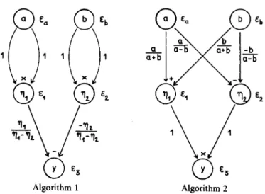
Error Propagation
The amplification factors (a + b)/(a + b + c) and 1, respectively, measure the effect of the rounding errors C1> c2 on the error cy of the result. Amplification factors for the relative errors are similarly associated with, and written along the arcs of the graph.
Examples
The algorithm is then numerically stable, at least as far as the effect of rounding error is concerned. The numerical stability of the above algorithm is often demonstrated by interpreting (1.4.1 O) in terms of backward analysis: Calculated approximate solution b.
Interval Arithmetic; Statistical Roundoff Estimation
We denote the expected value by Jie and by a; the variance of the upper bound distribution. The first of the above formulas follows the linearity of the expected value operator.
Interpolation
Interpolation by Polynomials
The upper expansion coefficients are located in the upper descending diagonal of the divided difference scheme (2.1.3.7). All Newtonian representations of the above kind can be found in a single divided difference scheme, which arises if they support the arguments Xi'.
Interpolation by Rational Functions
D Note that the converse of the above theorem does not hold: a rational expression <111 may well solve SIl, v, whereas some equivalent rational expression-. D The observation (2.2.1.8) makes it clear that the insolvability of the rational interpolation problem is a degeneracy phenomenon: the solvability can be restored by arbitrary small perturbations of the support points. Most of the following discussion will be about recursive procedures for solving rational interpolation problems Am.
We now assume that p~; f, v-1 =1= 0, and multiply numerator and denominator of the fraction above by.
Trigonometric Interpolation
In the following pseUdO-ALGOL formulation of the classical Cooley-Tukey method, we assume that the set P[ ] is initialized by setting To overcome these numerical difficulties, Reinsch modified Goertzel's algorithm [see Bulirsch and Stoer (1968)]. The latter only causes the following error L\).sl in sl:. In practice, often all one knows about a function are its values./k := J(Xk) in equally spaced arguments xk:= 2nk/N, where N is a given fixed positive integer. The problem is to find, under these circumstances, reasonable approximate values for the Fourier coefficients cAf).
As a by-product of the above proof, we obtained an explicit formula (2.3.4.8) for the attenuation factors.
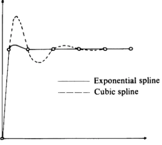
Interpolation by Spline Functions
We will confirm that each of these three conditions by itself ensures uniqueness of the interpolating spline function S&(Y;). We will show that spline functions are readily characterized by their moments, and that the moments of the interpolating spline function can be calculated as the solution of ' n system of linear equations Note that the second derivative S:\(Y; .) of the spline function coincides with a linear function in each interval [Xj' Xj+l],j = 0,.
First, we will show that the moments (2.4.2.1) of the spline interpolation function converge to the second derivatives of the given function.
Topics in Integration
The Integration Formulas of Newton and Cotes
Additional integration rules can be found by Hermitian interpolation (see Section 2.1.5) of the integrand f with a polynomial P E ITn of degree n or less. The full integral is then approximated by the sum of the approximations of the subintegrals. When decreasing the step length h (increasing N), the approximation error approaches zero as fast as h2 , so we have a method of order 2.
By replacing j'(a),f'(b) by difference quotients with an approximation error of sufficiently high order, we obtain simple modifications ["end corrections": see Henrici (1964)] of the trapezoidal sum that does not involve derivatives. but still results in methods of orders higher than 2.
Peano's Error Representation
Before proving the theorem, we will discuss its application to the case of Simpson's rule. This then shows that the entire Rx operator moves by integration and we get the desired result. Note that Peano's integral error representation is not restricted to operators of the form (3.2.1).
In general, the Newton-Cotes formulas of degree n integrate without error polynomials P E TIn if n is even and P E TIn + 1 if n is odd (see Exercise 1).
The Euler-Maclaurin Summation Formula
In this form, the Euler-Maclaurin summation formula expands the trapezoidal sum T(h) in terms of the step length h = (b - a)/N, and therein lies its importance for our purposes: the existence of such extension puts a wide arsenal of powerful general "extrapolation methods" at one's disposal. We will use integration by parts and determine polynomials Bk(x) successively, starting with B 1 (X) == X - t, such that.
Integrating by Extrapolation
The above result (3.4.2) shows that the error term of the asymptotic expansion (3.4.1) becomes small compared to the other terms of (3.4.1) as h decreases. The expansion then behaves as a polynomial in h2 which gives the value of the integral for h = O. For the sequence (3.4.5a), half of the function values needed to compute the trapezoidal sum T(hi+ d) have been encountered before in the calculation of T(hi ), and their recalculation can be avoided.
Such an approximation s can be obtained simultaneously with calculating one of the trapezoidal sums T(hJ). A more general stopping rule will be described, together with a numerical example, in Section 3.5.
About Extrapolation Methods
We will see later that the central difference coefficient is a better approximation to base the extrapolation method on, in terms of convergence, because its asymptotic expansion contains only powers of the step length h. For the following discussion of discretization errors, we will assume that 1;k(h) are polynomials with exponents of the form Yk = kyo The Romberg integration (see Section 3.4) is a special case with y = 2. We are now able to used the asymptotic expansion (3.5.1) which gives for k < m.
Note that increasing the order of convergence from column to column which can be achieved by extrapolation methods is equal to 'Y: 'Y = 2 is twice as good as 'Y = 1.
Gaussian Integration Methods
Note that the abscissas Xi must be mutually distinct, since otherwise we could formulate the same integration rule using only n - 1 of the opposing abscissas Xi' (3.6.12c). We will examine this problem under the assumption that the coefficients (ji' Yi of the recursion (3.6.5) are given. In section 5.5 it will be seen that the characteristic polynomials Pj of Jj complete the recursions (3.6.5). with the matrix elements bi, Yi as coefficients.
Since v(ilT v(il = (Po, Po) by hypothesis, we obtain Wi = (vy»)2. D If the QR method is used to determine the eigenvalues of In, then the first components vY) of the eigenvectors vIi) are calculated is easily included in this algorithm: calculating the abscissa Xi and the weights Wi can be done simultaneously [Golub and Welsch (1969)].
Integrals with Singularities
If the new integrand is singular at 0, one of the above approaches can be tried. By construction, the nth Newton-Cotes formula yields the exact value of the integral for integrands that are polynomials of degree at most n. Iff E C2[a, b] then there exists an X E (a, b) such that the error of the trapezoidal rule is expressed as follows:. b) By construction, the above formula represents an integration rule that is exact for all polynomials of degree 5 or lower.
What is the form of the tridiagonal matrix (3.6.19) in this case. In the Chebychev case, the weights Wi are equal for general n.) 19.
Systems of Linear Equations
Gaussian Elimination. The Triangular Decomposition of a Matrix
As can easily be seen. with permutation matrices Pj and non-singular Frobenius matrices Gj of the form. Thus, using the Gaussian elimination algorithm, it can be shown constructively that every square non-singular matrix A has a triangular decomposition of the form (4.1.9). In the case that P = J, the pivot elements rii are representable as quotients of the determinants of the most important minors of A.
A further practical and important property of the triangular decomposition method is that for band matrices of bandwidth m,.
The Gauss-Jordan Algorithm
In the transition AU-I) ----+ AU) the variable Xj is replaced by Yj. Thus, AU) is obtained from A(j-l) according to the rules below. For simplicity, the elements of AU-I) are denoted by ailo and those of AU) by a;k'. a) Partial turn selection: Determine r so that.
The Cholesky Decomposition
All principal submatrices of a positive definite matrix are also positive definite, and all principal minors of a positive definite matrix are positive. The inverse of a positive definite matrix A exists: If this were not the case, an x =fo 0 would exist with Ax = 0 and xH Ax = 0, contrary to the definiteness of A. Now assume that the statement is true for positive definite matrices of order n - 1, and let A be a positive definite matrix of order n.
The lower triangular matrix L is stored in the lower triangular section of A, with the exception of the diagonal elements of L, whose reciprocals are in p.
Error Bounds
Clearly, lub(A) is the smallest of all the matrix norms IIAII which is consistent with the vector norm II x II. According to theorem (4.4.15), cond(A) also measures the sensitivity of the solution x of Ax = b to changes in the matrix A. Estimates obtained up to this point show the importance of the quantity cond(A) in determining the influence on the solution of changes in the given data.
Associated with each approximate solution x of the system Ao x = bo there is a matrix A E 'Jl and a vector b E !D satisfying.
Roundoff-Error Analysis for Gaussian Elimination
The sum of the absolute values of the elements in the rows (and columns) e. Assume that the rows of the n x n matrix A are already ordered such that A has a triangular decomposition of the form A = LR. For the matrix F, then, the inequality form the exact triangular decomposition of the matrix A - F, which differs slightly from A. Gaussian elimination is stable in this case. the partial selection of the pivot can easily be shown that ak-l ~2kao,.
For example, in the case of the Hessenberg matrices above, it is a shape matrix.
Roundoff Errors in Solving Triangular Systems
So far, no matrix has been found that does not satisfy. when using full pivot selection. In this section, we investigate the influence of rounding errors on the solution of such systems of equations. The calculated solution can therefore be interpreted as the exact solution of a slightly modified problem, which shows that the process of solving a triangular system is stable.
A comparison of (4.6.5) with the result (4.4.19) due to Oettli and Prager (1964) shows, finally, that the calculated solution x can be interpreted as the exact solution of a slightly modified system of equations, provided that the matrix n I [II R I has the same order of magnitude as I A I .
Orthogonalization Techniques of Householder and Gram-Schmidt