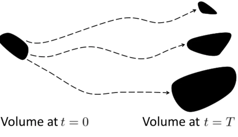
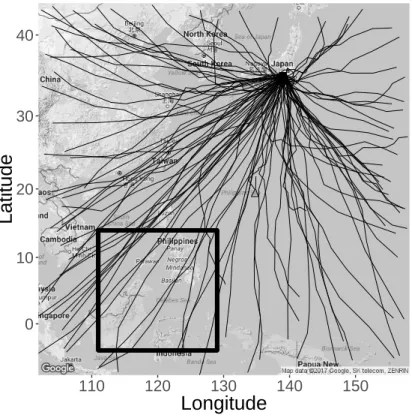
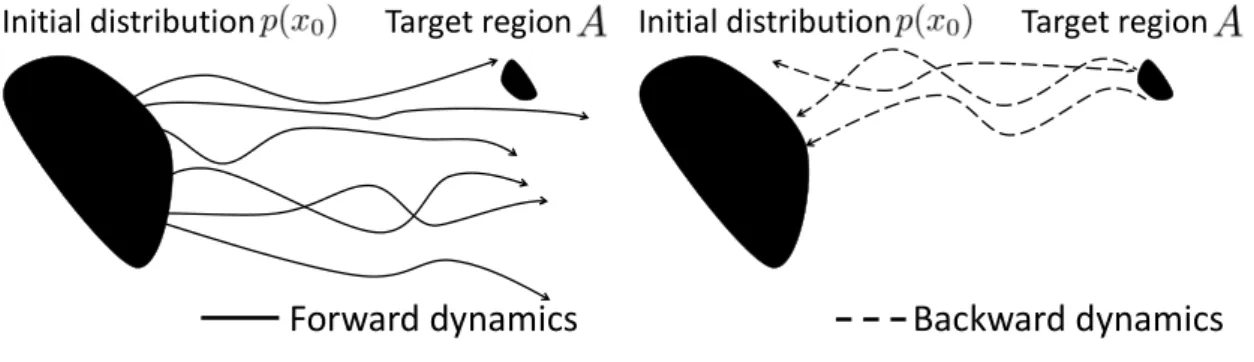
The forward simulation is inefficient when the target region A is much smaller than the support of the initial distribution p(x0). The backward simulation simulates paths from the target region A to the support of the initial distribution p(x0). The black rectangular region shows the possible initial position of typhoons in the northwestern part of the Pacific Ocean.
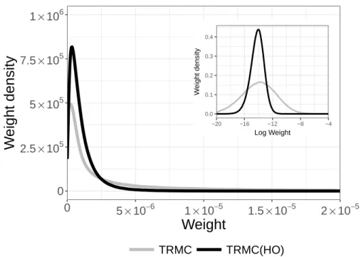
The black rectangular area corresponds to the possible initial position of typhoons in the northwest Pacific Ocean. The variance of the distribution by the TRMC (HO) is much smaller than that by TRMC.
Introduction
- Background
- Failure of Na¨ıve Method
- Derivation of Eq. (1.12)
- Sequential Importance Sampling
- Sequential Monte Carlo
- Time Reverse Monte Carlo Method
- Implementation for Stochastic Difference Equa- tion
- Derivation of Eq. (3.9)
The forward simulation is inefficient when the target regionA is much smaller than the support of the initial distribution p(x0). Moreover, the calculation of g−1 in Eq. 1.2) is time-consuming and reduces the efficiency of the calculation. We consider an estimate of the probabilityP(XN ∈A) that XN hits a small target region A in D-dimensional space.
1.4) Using this definition, we can rewrite Eq. 1.6) The probability calculated by equation 1.4) with i=N and ˜p(yi|yi+1) is the transition probability density from yi+1 toyi defined by the equation. In this chat, we describe the basic knowledge of Sequential Monte Carlo (SMC), as the time-reversal Monte Carlo (TRMC) method is based on the ideas of SMC. SIS corresponds to a generalization of the importance sampling (IS) technique for a sequence of distributions.
As we show in the next section, the resulting algorithm is simple but efficient compared to forward simulation when the target region A is smaller than the support of the initial distribution p(x0).
Applications
Stochastic Difference Equation
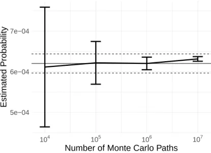
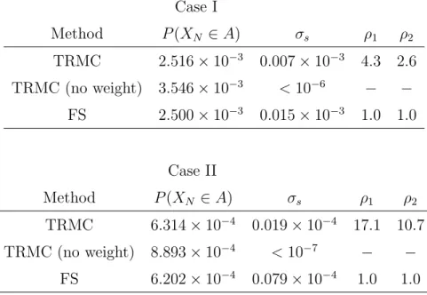
To demonstrate how the TRMC algorithm works, we first consider the two-dimensional stochastic differential equation that defines it. We set the number of Monte Carlo paths M to 107 and the number of time steps N to 10. This reveals that our algorithm gives unbiased probabilities compared to those calculated by FS.
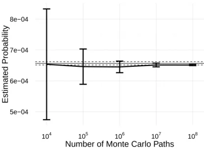
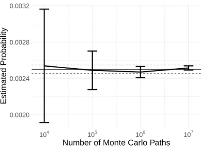
The line titled "TRMC (no weights)" means that we ignore the factor defined by equation (3.4) when evaluating the probability. The horizontal line in Figure 4.1 indicates the estimated probability by FS with the number of Monte Carlo paths M = 107. The horizontal dashed line in Figure 4.1 shows the ±1 standard error confidence intervals after the FS with the number of Monte Carlo paths M = 107.
It reveals that our algorithm converges correctly by increasing the number of Monte Carlo pathsM. The estimated probabilities converge to those obtained by FS as the number of Monte Carlo paths increases. The estimated probabilities converge to these probabilities in the forward simulation as the number of Monte Carlo paths increases.
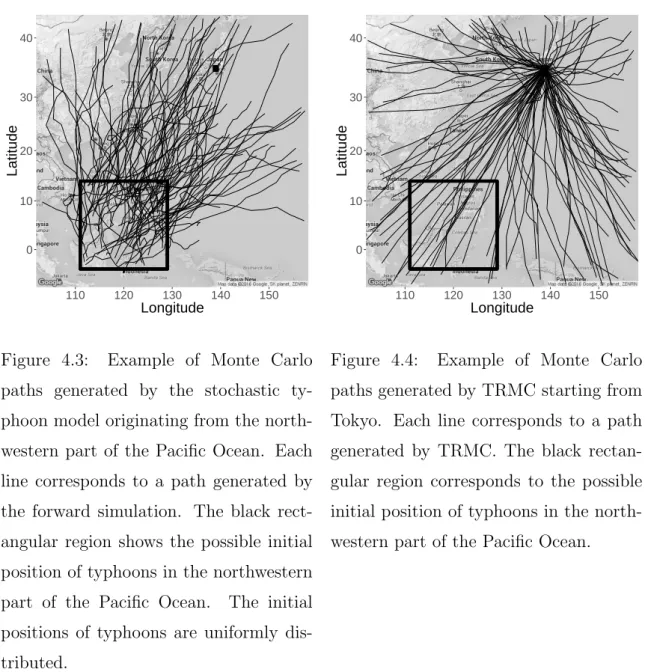
Stochastic Typhoon Model
The black rectangular area shows the possible initial position of typhoons in the northwest Pacific Ocean. The black rectangular area corresponds to the possible initial position of typhoons in the northwest Pacific Ocean. The computation time of TRMC in this simulation for generating 108 Monte Carlo paths is approximately 4.0 x 10³ seconds.
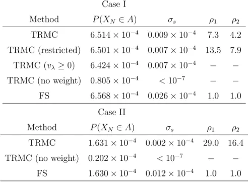
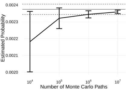
The estimated probabilities converge to those obtained by FS as the number of Monte Carlo paths increases. FS has the same number of Monte Carlo paths, M = 108, as TRMC. biased probability as in the case of the stochastic difference equation. To avoid this and improve its efficiency, we restrict the velocity distribution of Monte Carlo paths to the tendency to move southward.
As the number of unnecessary northward moving Monte Carlo paths is reduced, TRMC is (bounded) more efficient than TRMC. The stricter constraint vλ ≥ 0, however, causes a small bias in the estimated probabilities: see TRMC (vλ ≥0) in Table 4.2. For now, we consider the case where the number of time steps from the initial position to Tokyo is precisely known (N = 16).
A typhoon can pass close to Tokyo, for example between N = 15 and N = 16, causing an underestimation of the real risk when we only consider hits at integral time steps. The black rectangular area corresponds to the possible initial position of typhoons in the northwestern part of the Pacific Ocean. The estimated probabilities converge to those obtained by FS as the number of Monte Carlo paths increases.
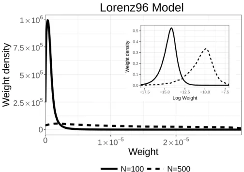
Lorenz 96 Model
While many discretization schemes are available, we focus on the simplest and most common scheme, the Euler scheme. The computation time of TRMC in this simulation for generating 107 Monte Carlo paths is about 3.0×10³ seconds. The case where we ignore the factor determined by Eq. 3.4) does not reproduce the same unbiased probability as other computational experiments.
The result shows that TRMC can perform better for estimating probabilities in the high-dimensional case. The estimated probabilities converge to those obtained by FS as the number of Monte Carlo paths increases.
Higher-order Approximation
The result is shown in Table 5.1 and shows that TRMC (HO) is much more efficient in this case. As we expect, the variance of the distribution under TRMC (HO) is smaller than that from TRMC, which leads to efficient estimation of probabilities.
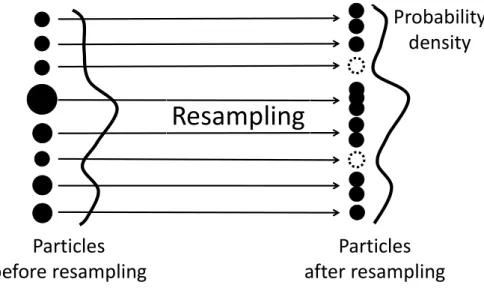
Resampling
Vertical and horizontal lines indicate weight density and weight value, respectively. Therefore, a resampling process is performed when this value is lower than a certain threshold Θ = αM, where α is a relative threshold. It shows that the probabilities of FS, TRMC and TRMC (RS,α=50%) agree within the error bars.
External Field
In this case we can transform the backward dynamics (3.6) as follows. 5.11) Hereafter we refer to TRMC with this backward dynamic as TRMC (EF). In TRMC (EF), the external field pulls the path toward a target area A. As a result, TRMC (EF) powerfully increases the probability of the simulation paths hitting a target area A.
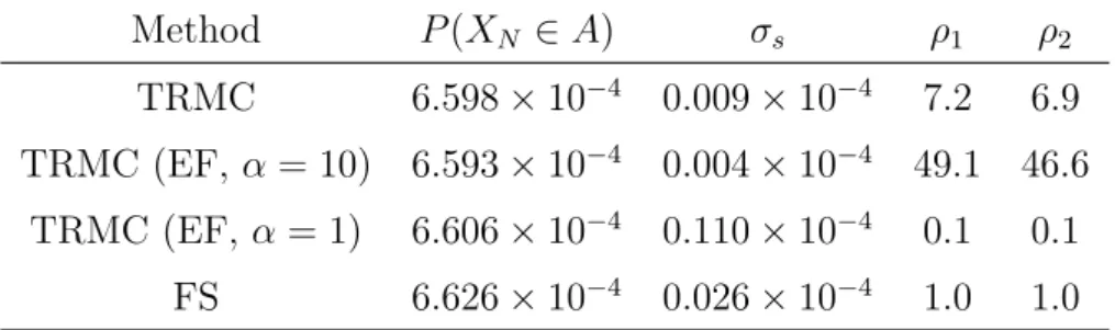
This shows that the probabilities of FS, TRMC and TRMC (EF,α = 10) agree within the error bars. On the other hand, TRMC (EF, α= 1) does not reproduce the unbiased estimates of the probability. This is because the strong external field compared to the support of the initial distribution p(x0) bias occurs.
TRMC (EF, α = 1) does not reproduce the unbiased probability estimates due to the strong external field. This shows that the number of hits tends to increase when α decreases as we expected. As one way, we can use α (and β) where the effective sample size Mef f is maximum.
The second way is to use the effective sample size ratio defined by the effective sample size Mef f divided by the number of hits. In this method, we can use α before the sharp drop in the effective sample size ratio. The effective sample size becomes largest when α = 10, which is consistent with the trend of computational efficiency.
Discussion
To discuss possible improvements to the algorithm, it is useful to introduce the optimal feedback dynamics. First, the marginal probability at step n obtained by forward simulation is defined as . 6.1) and (6.2), the transition probability q∗ of the optimal feedback dynamics is defined as 6.3) appears similar to the formulas used in Bayesian inference, when the probability p(xi) obtained by forward simulations is treated as an analogue of the prior distribution xi. 6.4) means that the total probability of the time-reversed trajectories defined by the forward simulation is recovered by the backward dynamics equation.
In particular, the time-reversed paths initialized by p(xN) automatically converge to their initial density p(x0) using the backward dynamics Eq. 6.3) is considered the optimal backward dynamics. Note that the backward dynamics defined by the Langevin equation in previous studies can be derived from Eq. Equations (6.3) and (6.4) have been discussed previously in the field of time series data analysis, using marginal probabilities approximations.
Methods such as those discussed previously [55, 56] can be used to optimize the feedback dynamics in our problem, but this is left to future studies. On the other hand, when some observed data are available outside the equations describing the stochastic process, these data can be used to approximate p(xi), i= 1,. In this case, we avoid using a large amount of forward computation to build the optimized backward dynamics.
Note that this idea is different from data assimilation (i.e., inference with simulations combined with observed data), because here we use observed data only to improve computational efficiency; they do not bias the calculated probabilities. 5.8) after realignment, the exact backward dynamics coincides with the optimal backward dynamics in the range of O(∆t) according to this approximation. Therefore, we can interpret TRMC (EF) as one of the methods of approximating the optimal backward dynamics.
Concluding Remarks
In the case of a realistic typhoon model, we need to consider the passage through Tokyo between two separate time steps. I(t) converges in probability if the mesh ||Π|| of the partition tends to zero if the limit exists. We can simulate the exact backward dynamics using a numerical method such as the Euler method.
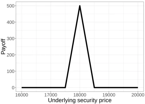
Estimating the correct value for these options is a fundamental and challenging problem in the financial industry. In this appendix, we assume that there is one underlying security and the discretized dynamics of the price process U ={U0, U1,. Monte Carlo methods are popular computational methods for estimating Eq. B.1), especially if the portfolio includes many options (portfolio of options) or if the underlying space has high dimensionality [64].
An important point in the practical financial risk management of an option portfolio is that the value of an option portfolio varies non-linearly. It is then possible to estimate how much loss in the value of a portfolio will occur when the financial market falls sharply. In the financial industry, it is common to calculate using a forward simulation, so we use FS as the basis in this appendix.
Since the payoff function introduced here can be described as a combination of call/put options, we can use Black-Scholes formula to calculate the exact solution of this simulation. Using these variables, as in the main text, we define a measure of the relative computational efficiencyρ2 as. This efficiency is defined in terms of the actual performance taking into account both the computation time and the variance of the resulting estimates.
Detection of information sources in the sir model: a sample path-based approach. IEEE/ACM Transactions on Networks (TON. Monte Carlo Filter and Smoother for Non-Gaussian Nonlinear State Space Models. Journal of Computational and Graphical Statistics.