arXiv:astro-ph/9809081v1 7 Sep 1998
T. W. Jones1, Dongsu Ryu2 and Andrew Engel1,3
ABSTRACT
We introduce a simple and economical but effective method for including relativistic electron transport in multi-dimensional simulations of radio galaxies. The method is designed to follow explicitly diffusive acceleration at shocks, and, in smooth flows, second-order Fermi acceleration, plus adiabatic and synchrotron losses for electrons in the energy range responsible for radio emission in these objects. We are able to follow both the spatial and energy (momentum) distributions of the electrons, so that direct synchrotron emission properties can be modeled in time dependent simulated flows of this type for the first time. That feature is essential if simulations are to bridge successfully the fundamental physical gap between flow dynamics and observed emissions.
As an initial step towards that goal, we present results from some axis-symmetric MHD simulations of Mach 20 light jet flows. These explicitly explore the effects of shock acceleration, as well as adiabatic expansion and synchrotron aging in smooth flows. The simulations demonstrate the importance of the fact that even for steady inflows jet terminal shocks are not simple, steady plane structures. Most importantly this should play a very major role in determining the properties of synchrotron emission within the terminal hot spot and in the lobes generated by the jet back flow.
In fact, the outflows are inherently complex, because of the basic “driven” character of a jet flow. Consequently, the nonthermal electron population emerging from the jet may encounter a wide range of shock types and strengths, as well as magnetic field environments.
We may expect to find a complex range in synchrotron spectral and brightness patterns associated with terminal hot spots and lobes. These include the possibility of steep spectral gradients (of either sign) within hot spots, the potential in lobes for islands of flat spectrum electrons within steeper spectral regions (or the reverse) and spectral gradients coming from the dynamical history of a given flow element rather
1Department of Astronomy, University of Minnesota, Minneapolis, MN 55455: [email protected]
2Department of Astronomy & Space Science, Chungnam National University, Daejeon 305-764, Korea:
3Department of Physics, University of Arizona Tucson, AZ 85721: [email protected]
4Accepted for publication in the Astrophysical Journal
than from synchrotron aging of the embedded electrons. Finally, synchrotron “aging”
in the lobes tends to proceed more slowly than one would estimate from regions of high emissivity. That is a consequence of the fact that those regions are ordinarily places where the magnetic fields are the strongest, so that the instantaneous rates of energy loss are atypical of the full history of the electron population. This feature supports earlier suggestions that nonuniform field structures may help to explain why dynamical ages of FRII sources often seem to be greater than the apparent age of the electrons radiating in the lobes, as measured in terms of spectral steepening, or absence thereof.
Subject headings: particle acceleration – galaxies: jets – magnetohydrodynamics: MHD – radio continuum: galaxies
1. Introduction
The standard paradigm for radio galaxies (RGs) is based on high speed plasma jets, formed in active galaxy nuclei (AGN), but penetrating far into circumgalactic environments and creating giant lobes of luminous material as a consequence of interactions with the intergalactic medium (e.g., Bridle 1992). The defining radio emission represents synchrotron radiation from relativistic electrons and magnetic fields. Those two crucial constituents are thought to be transported from the AGN, enhanced or generated by the jet-IGM encounter or both. Modern radio interferometry has provided richly detailed intensity, spectral and polarimetric images of RGs (e.g., Leahy et al. 1997), while rapidly advancing computational tools have allowed increasingly sophisticated multi-dimensional magnetohydrodynamical (MHD) simulations of the plasma flows (e.g., Clarke 1996). This paper presents the first such simulations that explicitly include time dependent transport of the relativistic electrons that produce the observed radio emission in such objects.
Coleman & Bicknell 1988 carried out an early related calculation by mapping an analytic electron distribution onto a simulated bow-shock flow pattern, while Jones & Kang 1993 followed the time dependent behavior of a simplified electron distribution during the evolution of a shocked gas cloud. Clarke et al. 1989 and Matthews & Scheuer 1990 computed early models of synchrotron emission from RGs based on simulated fluid dynamical variables and intelligent guesses at the possible relativistic electron properties. But, no published simulations have followed the full electron distribution through a time-dependent evolution in a simulated RG-like flow. That important feature is a very difficult technical challenge, because the length and time scales needed to model effectively the microphysics of electron transport are typically many orders of magnitude smaller than those convenient to include in full scale hydrodynamical or magnetohydrodynamical simulations of RGs.
To avoid these difficulties we introduce here a simple, economical method of relativistic electron transport that directly utilizes those mismatched scales and is suitable for time-dependent RG simulations. The method is designed to include the effects of diffusive shock acceleration and second-order Fermi acceleration, as well as adiabatic compression or expansion and synchrotron radiative cooling of the electrons in smooth flows. We present results of its initial application.
There are many dynamical effects that are likely to influence the eventual synchrotron brightness distribution and spectrum to be expected in realistic models of RGs. Before it makes sense to attempt anything that could be termed a “real” model of a RG, it is crucial that the individual dynamical influences be understood. The present paper, therefore, is intended to begin addressing these individual factors. The role of shock acceleration of RG electrons is centrally important (e.g., Heavens & Meisenheimer 1987; Blandford & Eichler 1987; Takarada 1989; Kr¨ulls 1992) While there are many studies of the physics of particle acceleration at plane or spherical shocks (e.g., Kang & Jones 1991), there are few previous simulations designed to explore shock acceleration in complex flows (but seee.g., Jones, Kang & Tregillis 1994) and, as mentioned, none for flows similar to those expected in RGs. Therefore, our first priority is to explore how shock acceleration may be characterized and recognized in such environments, or the degree to which
such flows may tend to confuse simple interpretations of this process.
Given these objectives and the fact that 2D, axis-symmetric flows are much easier to understand than 3D flows and still provide a first cut at the properties of RG flows, we limit this initial study to that problem. We have begun an extension of this work into fully 3D simulations and will present those results elsewhere. Since synchrotron cooling (commonly called
“aging”) is also likely to be a significant effect and will compete with and mask the influence of shock acceleration, we also include here an example of a flow that includes both of these effects together. We defer to later papers inclusion of second-order Fermi acceleration, not because it is necessarily unimportant, but because it is significantly more difficult to establish a unique, physical characterization of the momentum diffusion controlling it. Thus, at this stage, it would add significant complexity and uncertainty to an already complex set of questions.
The plan of the paper is this. In §2 we outline our methods, including the new electron transport scheme. Section 3 introduces the parameters of the jet flows we have modeled, while
§4 discusses our results. A brief summary of key findings is given in §5. An appendix contains a detailed discussion of practical requirements for numerical treatment of electron transport in RGs and justification for the scheme we introduce here.
2. Methods 2.1. Dynamics
We evolve the equations of ideal nonrelativistic magnetohydrodynamics (MHD) in cylindrical coordinates (r, φ, z), with φ an ignorable coordinate. All three components of velocity and magnetic fields are included, so the model is 212-D. The code is an MHD extension of Harten’s (Harten 1983) conservative, second-order finite difference “Total Variation Diminishing” scheme, as detailed in Ryu & Jones 1995; Ryu, Jones & Frank 1995; Ryu, Yun & Choe 1995 and Ryu et al. 1998. The code preserves ∇ ·B = 0 at each time step using an approach similar to the Constrained Transport (CT) scheme (Evans & Hawley 1988) as described in detail by Ryu et al. 1998a. We use a passive “mass fraction” or “color” tracer, Cj, to distinguish material entering the grid through the jet orifice (Cj = 1), or from ambient plasma (Cj = 0).
2.2. Electron Transport
Our electron transport scheme is an adaptation of the standard diffusion-convection equation for charged particles (e.g., Skilling 1975);
∂f
∂t = 1 3p∂f
∂p(∇ ·~u)−~u· ∇f+∇ ·(κ∇f) + 1 p2
∂
∂p
p2D∂f
∂p
+Q, (2-1)
where f(~x, p, t) is the isotropic part of the nonthermal electron distribution, κ is the spatial diffusion coefficient, D is the momentum diffusion coefficient, Qis a source term that represents the net effects of “injection” and radiative losses at a given momentum, p, while the thermal plasma velocity is ~u. This equation is valid for “fast” (superthermal) particles when scattering is strong enough to keep the particle distribution almost isotropic and is appropriate on lengths large compared to the particle scattering length itself.
The first term on the right accounts for adiabatic compression or rarefaction in the background flow. Eq. [2-1] is not valid within shocks, but when integrated across a velocity discontinuity, the first three terms account for “first order Fermi acceleration” at shocks, also known as “diffusive shock acceleration”. The fourth term allows for second-order Fermi acceleration resulting from particle interaction with Alfv´enic turbulence (e.g., Skilling 1975; Blandford & Eichler 1987).
As mentioned in the introduction and explained in detail in the Appendix, there is a severe mismatch between RG dynamical scales and diffusive transport scales that apply to eq. [2-1] for electron momenta relevant to radio synchrotron emission. That mismatch makes it impractical with conventional computational methods to solve eq. [2-1] as it stands to study electron transport in full RG flows. That is, the electron diffusive lengths and times are vastly smaller than those appropriate to the gasdynamics. The key physical fact is that the characteristic energy of electrons radiating synchrotron emission can be stated roughly as E ∼3 ν
1
92/B
1
102 GeV, where ν9 is the observed frequency in GHz, and B10 is the magnetic field compared to 10 µG or nT. Thus, the electrons of interest mostly have energies<∼10 GeV (p<∼104 mc). The gyroradius of such particles isrg∼3×10¹¹EGeV/B10 cm. This leads to characteristic diffusion lengths and shock acceleration times in RGs<∼AU and<∼ yr, respectively compared to flow scales typically measured in kpc and kyr or larger. The most serious consequence of this comes from the requirement that numerical shocks must appear thinner than a particle diffusion length for accurate solutions of eq. [2-1] (see the Appendix).
However, as also explained in the Appendix, that same mismatch can be exploited to develop a simplified equation of electron transport, provided f(p) is sufficiently broad that it can be represented as a piecewise power law over finite momentum bins. This last feature is very natural, in fact, in light of the same small time and length scales for electrons, since very rapid diffusive shock acceleration guarantees that GeV electrons emerge from shocks with power law momentum distributions on time scales much less than time steps required by the MHD. For much higher electron energies these simplifying conditions break down, but the method we derive could be used to provide a “low energy injection spectrum” for those particles, as well.
For continuity with the remainder of our discussion we present here the simplified transport equation, but refer readers to the Appendix for derivation details and tests of its validity. We divide the momentum range of interest into a modest number, N, of logarithmically spaced bins bounded by p0, . . . , pN. Definingyi = lnpi/p0, bin widths can be expressed as, ∆yi =yi+1−yi = lnpi+1/pi. We can integrate equation [2-1] within each momentum bin to defineni = 4πRppi+1
i p3f dlnpas the
number of electrons in the bin. For convenience we normalizeni by the total plasma mass density, to form bi =ni/ρ, then assume a piecewise power law f(p) =fi (p/pi)−qi within pi ≤p≤pi+1, so that ni is given in terms of fi, qi and ∆yi by eq. [A2]. For these relatively low energies diffusive transport at shock discontinuities is properly handled by defining the form of the electron distribution just down stream of a shock to be the steady state power law appropriate to the jump conditions for that shock. That fixes the ratio bi+1/bi at shocks. Electrons are injected from the thermal plasma at shocks using a common injection model, so that a fixed fraction,ǫ, of the total electron flux through a shock is injected and accelerated to the appropriate power law momentum distribution. Away from shocks, in smooth flows, but where the diffusion lengths of the electrons are much smaller than dynamical lengths, spatial diffusion is negligible. We can easily include the effects of synchrotron “aging”. When all of these features are included eq. [2-1] becomes (see also eq. [A2])
dbi dt = 4π
1
3∇u−qD p2 + 1
τso
p ˆ p
p3f ρ
pi+1
pi , (2-2)
where τso = 34σ(mc)2
TUB
1 ˆ
p defines the synchrotron cooling time at momentum ˆp, which we take arbitrarily to be ˆp = 104 mc. In this expression, σT is the Thomson cross section, and UB =B2/(8π). Note that the right hand side of eq. [2-2] is the difference between fluxes at the two momentum boundaries of the bini. Thus, we have a conservative, finite volume scheme that depends on a simple model of sub-grid structure (in momentum space) for its accuracy.
Although straightforward to include, we now drop the second order Fermi term, “D” from these initial simulations for the following reasons. First, in the vicinity of shocks, this acceleration process is likely to be much less efficient than first-order Fermi acceleration. That is simply because the second-order process comes from nearly balanced energy fluxes of waves propagating parallel and antiparallel to the magnetic field that resonantly scatter with the electrons; i.e.,on
“isotropic” Alfv´enic turbulence. First-order Fermi acceleration, on the other hand, depends only on waves propagating in the streaming direction that will be generated by the streaming particles themselves. In either situation resonant waves have wavelengths comparable to the particle gyroradius. Downstream of the shocks where particle streaming may be less important, it is significant for such low particle energies that the resonant wavelengths are probably within a couple orders of magnitude of thermal ion gyroradii (taking us ∼108 cm s−1). Such waves may be fairly strongly dissipated, for example, by nonlinear Landau damping (e.g., Lee & V¨olk 1973).
Thus the level of relevant isotropic Alfv´enic turbulence will likely depend on a local cascade of hydrodynamical turbulence (e.g.,Grappinet al. 1982). While we will certainly want to understand what role post-shock, second-order acceleration might play (e.g., Borovsky & Eilek 1986; Kr¨ulls 1992), only ad hoc models could be applied at present. Since this set of computations represents the first effort to treat nonthermal electron transport inside time dependent models of RGs, and since there are many possible competing influences to be understood before “realistic” models are sensible, the best initial strategy is to restrict ourselves to the most straightforward physics that is likely to be important. First-order acceleration is efficient and almost certain to happen at shocks, so its role must be understood from the beginning.
2.3. Computation of Synchrotron Emissivity
From the spatial distribution of bi and qi along with the MHD variables, ρ and B, it is straightforward to compute the synchrotron spectral emissivity, jν. Ignoring corrections due to slow curvature in the electron spectrum,jν, can be expressed as (cf. Jones, O’Dell & Stein 1974)
jν =jαo4πe2 c f(p)pq
νB⊥
ν α
νB⊥, (2-3)
withα = q−23,jαo ∼1 (cf. Jones, O’Dell & Stein 1974) and νB⊥=νBcosθ the electron cyclotron frequency in terms of the magnetic field projected over the angle θ onto the plane of the sky.
f(p) along with q are found from mapping bi and qi onto the critical synchrotron frequency as p =mcq3ν2ν
B⊥. We have interpolated q between momentum bin centers to give α a continuous form. Eq. [2-3] would break down for strongly curved spectra, but by that point in calculations of the type used here the local index will be too steep for the emission to be significant. In a calculation designed to predict the surface brightness distribution of a RG model one should include explicitly the effects of variations in cosθ. That is not our intention here, and such a calculation would need to evaluate carefully the effects of “sub-grid” fluctuations in the field directions and of the orientation of the jet with respect to the line of sight. Our aim here is to understand how electron acceleration and transport are likely to be reflected in the overall emission properties of a region within a RG, independent of the location of the observer. For those purposes it is better to ignore the factor cosθ, so will in this paper simply take it to be unity. Again, we are not in this paper computing surface brightness distributions from these simulations, which would involve line-of-sight integrations of jν. That would be inappropriate, given the axis-symmetric nature of the simulations, and would further exaggerate the dynamical constraints imposed by this symmetry.
3. The Simulated Jet Properties
Our initial simulated MHD jets are all dynamically identical. They have a simple, “top hat”
velocity profile, are Mach 20 with respect to the uniform ambient medium (Mj =uj/ca = 20), in thermal pressure balance with it, and have a density contrast η =ρj/ρa = 0.1. The jet enters at z = 0, with an initial radius of 36 zones, while the entire uniform grid is 384×1536 zones (1023rj×4223rj). Defining length and time in units of initial jet radius (rj = 1) and ambient sound speed (ca =pγPa/ρa = 1, with γ = 53), the simulations are followed for about 11.7 time units, when the bow shock of the jet reaches the rightz boundary. Reflecting boundaries are used along the jet axis, while continuous boundaries are used elsewhere. There is a background poloidal magnetic field (Bbackground) (Bφ = Br = 0; Bz = Bzo), with a magnetic pressure 1% the gas pressure; i.e., Pb = β1P, with β = 102. The in-flowing jet carries an additional toroidal magnetic field component appropriate to a uniform axial jet current with a return current on the surface of the jet; i.e., Bφ = 2×Bzo(r/rj) for r ≤rj. At r =rj, β = 20. The in-flowing jets are slightly
over-pressured at the outside.
These simulations are truly MHD rather than HD, despite the apparent weakness of the initial magnetic field. Even at the initial strengths modeled here the magnetic fields play a role in the evolution, especially in the cocoon. There are numerous locations where the plasma β ∼10, so that its pressure is not entirely ignorable. There is, however, a more important and much less recognized role for the field in flows initialized with even β >>1. In 2-D and 3-D MHD simulations of the Kelvin-Helmholtz instability, for example, we have demonstrated crucial dynamical contributions from magnetic fields in flows with initialβ >103 (e.g., Jones et al. 1997;
Ryu et al. 1998b; Jones, Ryu & Frank 1998). The point is that through field “stretching”, magnetic tension can be increased in complex flows to the point where it is comparable to or exceeds the Reynolds stresses of the gasdynamical flow ( coming from spatial variations inρuiuj), even though the magnetic pressure may be smaller than the gas pressure. The relative importance of Maxwell to Reynolds stresses can be roughly represented by the Alfv´en Mach number in a flow, MA =u/vA. When the local MA drops to small values in a complex flow, that can lead through reconnection to so-called “dynamical alignment” and flow “self-organization”. There are also many locations within our model flows whereMA<∼1. In short, the flows are made smoother by the presence of the field, even though in the original configuration the field nominally appeared too weak to influence the dynamics. A comment may be in order on the meaning of magnetic reconnection obtained from an “ideal MHD” code. While reconnection is most fundamentally a topological transition (e.g., , Axford 1984), it cannot take place without resistive, dissipative effects on small scales. In an ideal MHD code these dissipative effects are numerical in origin, so we cannot model the microphysics of driven reconnection (which is still not understood at this time, in any case). However, there is evidence that the phenomenology of reconnection is often correctly captured. For example, Miniatiet al. (1998), using the Cartesian version of the code we employ here, demonstrate clear development in 2-D supersonic MHD cloud simulations of the so-called
“resistive tearing-mode” instability that is physically associated with driven reconnection.
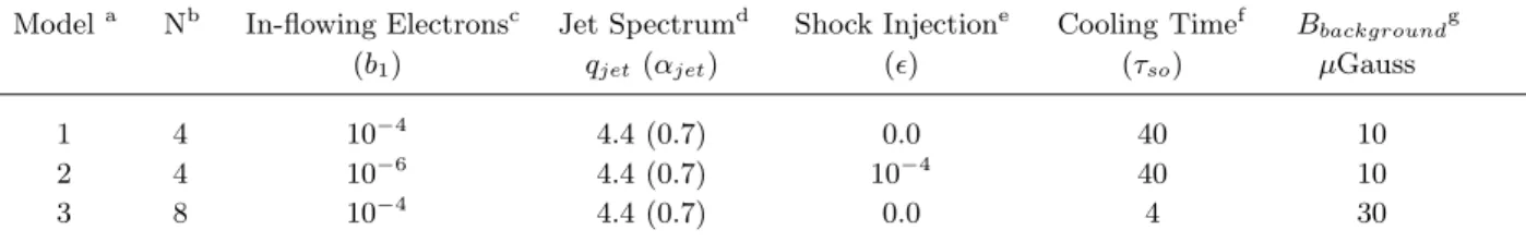
We present here three examples of the electron transport within the dynamics of the above jet flows. Their properties are listed in Table 1. Electrons are modeled in the momentum range p0 =mec and pN ≈1.63×10⁵mec. All three include the effects of diffusive shock acceleration.
Models 1and 2 are alike in that the electrons have negligible influence from synchrotron aging , while Models 1 and 3 are alike in that the electron populations originate entirely with the in-flowing jet. Model 2 differs in that the electron population is mostly injected locally from thermal plasma at shocks within the modeled flow. Model 3 differs, then, in that electrons are influenced very significantly by synchrotron aging.
In the “adiabatic” Models 1 and 2, there is very little curvature to the electron spectra, so in those models we used four momentum bins (i.e., N = 4) giving lnpi+1p
i = 3. (See the Appendix for justification of these numbers.) InModel 2we injected electrons at p0 using the simple model described in§A.3. Electrons should be injected at slightly suprathermal postshock energies, so the valuep0 =mecwas selected as appropriate for jets with speed uj ∼0.1c, assuming that shocked
Table 1. Summary of Simulations
Modela Nb In-flowing Electronsc Jet Spectrumd Shock Injectione Cooling Timef Bbackgroundg
(b1) qjet(αjet) (ǫ) (τso) µGauss
1 4 10−4 4.4 (0.7) 0.0 40 10
2 4 10−6 4.4 (0.7) 10−4 40 10
3 8 10−4 4.4 (0.7) 0.0 4 30
aAll models used Mach 20 jets (Mj =uj/ca = 20), with a density contrast, η=ρj/ρa = 0.1. Units come from a jet radius,rj = 1, an ambient density, ρa = 1, and a background sound speed, ca =p
γPa/ρa = 1 (γ = 5/3).
The cylindrical computational box was 10.67 rj units high and 42.67 rj long. End time for each simulation was t = 10.67 units. There was a uniform, poloidal jet magnetic field, Bz0 that also extended to the background, so Bz0=Bbackground withβ=P/Pb= 100, while the incoming jet also contained a toroidal field,Bφ= 2×Bz0(r/rj).
bNumber of electron logarithmic momentum bins spanning the range p0 = 1 mc to pN = 1.63×10⁵ mc.
(lnpN/p0= 12)
cRatio of nonthermal to thermal electrons in the incident jet flow.
dqjetis the momentum distribution power law index of the in-flowing electron population;αjetis the corresponding synchrotron index.
eAssumed fraction of the thermal electron population injected to the nonthermal population as it passes through a shock.
fTime for electrons to cool below momentum, ˆp= 104mc in the ambient, or background, magnetic field, measured in time unitsrj/ca.
gField that would produce the listed cooling time, assuming illustrative values for the simulated jet: uj = 0.1c, rj= 1 kpc. This would also map the displayed synchrotron emissivity data onto 1.4 GHz. Applying the additional constraints on the jet listed above, the implied jet density and kinetic luminosity are ρj ≈3×10⁻²⁹Bbackground2 g cm−3 andKkinetic=π2ρju3jrj2≈1.2×1043Bbackground2 erg sec−1, withBbackground inµGauss.
electrons are thermalized to a temperature comparable to but smaller than the ions. Since the nonthermal, cosmic-ray electrons are passive, all results could be scaled for different choices of p0.
To include synchrotron aging it is necessary to relate the characteristic cooling time τso defined in association with eq. [A3] to the computational time units, here given by rj/ca. The cooling time depends as well on the magnetic field strength and the momentum pas
τs = 2.5×101 1 p4
uj8 Mj
1 rjk
1
B102 , (3-1)
where τs =τsoppˆ, p4 is the electron momentum in units 104 mc, uj8 is the jet speed expressed in units of 108 cm s−1, Mj is the jet Mach number (here set to Mj = 20), rjk is the incoming jet radius in kpc, and B10 is the strength of the magnetic field in units of 10 µG, or equivalently in units nT. By comparison, the end points of our simulations aret= 1023.
For Models 1and 2 we have set τso = 40, the objective being to produce negligible aging for electrons of interest during the simulation. To project emission from electrons with momenta p<∼104 mc into the radio band, we should be considering magnetic fields>∼10 µG. Assuming, for example, thatBz0= 10µG, and uj8= 30, then rjk≈1.1, so that the length of our computational box would be about 45 kpc, and the time unit,rj/ca≈7×105 years.
By contrast, forModel 3we set τso= 4.0, so that synchrotron aging is now very significant for electrons in the energy range of interest over the time scale of the simulation. Keeping the same physical jet speed and radius, as well as the time unit, this case would correspond to an axial magnetic field Bz0 ≈30 µG. Other associated dependent parameters are outlined in Table 1. These combinations are illustrative only and not meant to be particularly representative of any real RGs. Other combinations would work as well for our present purposes, which are aimed at the physics of the electron transport. For the simulation of Model 3, we used eight momentum bins (N = 8) to cover the same range as the other models, as justified in §A.4.
4. Discussion 4.1. Flow Dynamics
We first outline some key dynamical properties of the simulations, remembering that the MHD properties of the different electron transport models are identical except for dimensional scaling factors. Fig. 1 shows at t = 10.67 images of the plasma density, ρ, the magnetic field intensity, B, and gas compression, dlndtρ =−∇ ·~u. The compression highlights shock structures.
These images remind us that such flows are complex and unsteady. All of the structures are ephemeral or at least highly variable. Jets, as strongly driven flows arenot reasonable to model as equilibrium structures (cf. Satoet al. 1996). As described by many before us (e.g., Norman, Smarr & Winkler 1985; Lind et al. 1989), once equilibrium is broken, jet plasma alternately expands and then refocuses while interacting with its self-generated cocoon, creating oblique jet
shocks as a result. 5 Those shocks are neither steady nor stationary, however. Most important to our discussion, the oblique jet shocks interact episodically with the terminal jet shock, causing it to vary in both strength and structure. The jet never re-establishes an equilibrium in its flow.
The terminal shock also includes a “Mach stem”, so that in 2-D at least, jet flow coming down the outside of the jet, nearrj, always exits through an oblique shock. At times there is little or no perpendicular terminal shock; then, most of the emerging jet flow is only weakly shocked. When a perpendicular portion to the terminal shock exists, it usually is strong, with a compression ratio σ ≈ 3.8 (→ q ≈ 4.08;α ≈0.54) in these simulations. The many other shocks and the oblique segments of the terminal shock are mostly weak (Fig. 1c), but they can exhibit density jumps, σ ∼>2−3 (→ q ≈6−92). Along the jet axis intersecting oblique shocks can be strong, but these intersections intercept a small fraction of the flow, so will not produce a large population of flat spectrum electrons.
Vorticity is shed from the outer edge of the terminal shock to form the turbulent jet cocoon.
There are distinct episodes of strong “vortex shedding” coincident with disruption and reformation of the terminal shock. Once shed, the vortices interact with the Kelvin-Helmholtz unstable boundary layer of the jet, generating an even more complex back-flow and perturbing the jet flow, as well. All of these dynamical features are represented in the Fig. 1. snapshot. The large “rolls”
visible in Fig. 1 are remnants of vortex rings that were shed earlier than the time displayed. The magnetic field in the back-flow is dominated within an axis-symmetric flow by Bφ, both because this magnetic component is enhanced by stretching in the expanding flow emerging from the jet, and because magnetic reconnection of theBr,Bz field components annihilates most of that field from the back-flow in an axis-symmetric geometry. This flux annihilation inside vortical flows is well-known and sometimes termed “flux expulsion” in the MHD literature (Weiss 1966). In a 3-D flow both the vortex and magnetic field structures would be stretched, twisted and tangled;
i.e., the back-flow would become turbulent and disordered on small scales (e.g., Norman 1996;
Ryuet al. 1998b; Jones, Ryu & Frank 1998) leading to vortex and magnetic flux tube complexes.
4.2. Electron Transport & Emissivity
The electron transport we model takes place “on top of” this dynamics;i.e., , the electrons do not feed back dynamically on the flow. To check this for consistency we confirmed that for the numbers we assume, the electrons never represent more than about 0.1 % of the kinetic energy density in the jet or the back flow. Remember that the dynamics behind the electron transport and synchrotron simulations discussed below is identical in each model. The electron distribution, and especially its momentum dependence, reflect the flow history of a given fluid element as appropriate for the particular transport assumptions, as well as the current fluid condition. Our
5In this paper “oblique” and “perpendicular” refer to the angle between the shock face and the velocity field, not the shock normal and the magnetic field, as is customary in the particle acceleration literature.
objective in this paper is to begin to learn how to interpret the emergent patterns. Since the astronomical tool for this is synchrotron emission, we will explore the physics in that paradigm using local emissivities. We expect that this approach will make much more tractable the interpretation of full 3D simulations. For the convenience of the discussion we express emissivities as they would be at 1.4 GHz, based on the fiducial magnetic field values listed at the end of §3 and in Table 1. They can be easily rescaled by choosing other combinations of source parameters.
Illustrative examples of the emissivity properties in these models are shown in Fig. 2 - 4. Fig. 5 explores the correlations between emissivity, spectral index and magnetic field strength using the same data displayed in the other figures. At the start we point out the obvious “limb brightening”
of the emissivities seen in all of the models displayed. This feature is not characteristic of real radio lobe surface brightness in FRII sources, but is an artifact of the assumed axis-symmetry of the simulations; particularly the persistence of the large “rolls” in the back-flow and the decoupling that occurs in axis-symmetry between Bφ and (Br, Bz). In an equivalent 3-D simulation the bright structures should be better mixed into the turbulent interior regions of the back-flow. This is one reason we defer any display of model surface brightness until we have 3-D structures in the models. That does not detract from the present discussion, however, since this initial exploration is mostly aimed at identifying physical relationships in emission properties and flow properties, as well as recognizing emissivity characteristics that we may eventually be able to use as diagnostics of the history of the local electron population.
4.2.1. “Adiabatic” Models 1 and 2
Fig. 2a and 2b provide grayscale images of logjν at 1.4 GHz for the “adiabatic” electron models1 and 2 at t= 10.67. For these two models emissivity values from eq. [2-3] are displayed when they are within a factor 3×10³ of the peak emissivity. Smaller emissivities are blacked out.
For comparison we also display with the same dynamic range in Fig. 2c a “pseudo emissivity”, based on the MHD properties of the flow; i.e., jc = CjP B32, modeled after the approach introduced in Clarke et al. 1989. We have added the jet color variable, Cj to Clarke’s original definition, because of differences in our assumed background magnetic field. Clarke’s magnetic field vanished outside the jet flow and its cocoon, whereas we used a simpler model that continues the axial field into the background. Since Cj = 0 in the background our definition allows jc >0 only for regions containing jet plasma, so that they are comparable to Clarke’s. On the other hand, for the Model 1,2 and 3 emissivities based explicitly on transported relativistic electrons, the absence of a significant electron population in the background makes this factor immaterial.
Fig. 3a and 3b show with an inverse gray scale the 1.4 GHz spectral index distributions, α =−∂logjν/∂logν|1.4 = (q−3)/2, (α1 and α2) over the same emissivity range in Models 1 and 2.
Fig. 2 compares emissivities produced by the two “adiabatic” models represented byj1 and j2. to the “pseudo emissivity”, jc. The three emissivity images have clear similarities. All show
a dominant “hot spot”, down stream (to the right) of the jet terminal shock. Each produces qualitatively similar patterns of bright emission within the back-flow. The jet is illuminated in the jc model emissivity with patterns that resemble those of the j1 model. Of course, the jet is largely invisible in j2, because the jet electron population is assumed very small in that model.
The model congruencies reflect the strong roles of two key ingredients to the emissivity; namely, the strength of the magnetic field and adiabatic compression and expansion. Note, however, that j1 and j2 have much greater local contrast than jc. Since the magnetic field distributions are identical for all three emissivity calculations, differences in the effective radiating electron distributions must be responsible. That is apparent by noting within smooth flows thatni ∝ρqi3, soj1,2 ∝niBqi2−1 ∝ρqi3 Bqi−12 . This is actually rather similar tojc ∝ρ5/3B3/2, except for variations modeled in bi =ni/ρ and qi, but not modeled by jc. The formula given for jc is based on an assumed α = 0.5, so contrast could be increased in jc by assuming a significantly steeper index.
The natural extension of jc to general α would be jc ∝ p2αρ1−2α(Bsinψ)α+1ν−α (D. Clarke, private communication). For α = 1 this gives jc ∝ (P B)2/ρ, just as for j1,2 with α = 1. That would not represent the same effect noticeable inj1 and j2, however, since from Figs. 2, 3 and 5, we can see that large j1,2 come primarily from regions whereα <0.7.
4.2.2. “Synchrotron Aged” Model 3
In Fig. 4 we show the analogous simulated synchrotron emissivity and spectral information for our Model 3, which includes the effects of synchrotron aging . Recall that, except for this influence, Model 3 is identical to Model 1. Thus, Fig. 4a (j3) can be compared to Fig. 2a (j1), while Fig. 4b (α3) can be compared to Fig. 3a (α1). In addition, we illustrate the level of spectral curvature of Model 3 in Fig. 4c, using of the difference between the simulated spectral indices at 1.4 GHz and 5.0 GHz (δ3 = α3(5GHz)−α3(1.4GHz)). Note that we use formal definitions of α rather than the traditional observed value defined by the ratio of fluxes measured at two distinct frequencies. The intrinsic “observed” index can be found by the simple formula α1.45 =α+ 0.5∗δ3. These “observed” indices would be almost the same asα near the origin of the jet and in flows just either side of the terminal shock in Fig. 4. On the other hand the “observed”
spectra would tend to be ∼0.05 steeper in mid regions of the jet and in most of the back flow, cocoon regions bright enough to show in this figure. But, we mention another caveat with regard to comparisons with directly observed properties. Beyond other complications already mention, including differences between emissivity and surface brightness, a real observation would likely smooth over a physically significant range of sight lines. Non-black regions in Fig. 4 cover a wider range of emissivity values (namely a factor 3×10⁴) than in Figs. 3 and 4, since the inclusion of synchrotron aging adds considerable contrast to the emissivity distribution. This factor 10 extension captures approximately the same physical regions as for the other models.
The emissivity distribution, j3, for Model 3 including synchrotron aging, is shown in Fig.
4a. As mentioned earlier, the dynamical range found in j3 is greater than for any of the other
models, since there is considerable steepening visible in the spectral index as one moves away from electron sources; namely, the jet origin and strong shocks. Steepening due to aging is apparent even within the jet, where α3 increases from 0.7 at the origin to values near 1 even before the first oblique shocks are encountered. Although the emissivity distribution within the jet in Fig. 4a is very similar in appearance to that forModel 1in Fig. 2a, the factor 10 increase in dynamic range covered in Fig. 2a slightly de-emphasizes the stronger emissivity decreases caused by synchrotron aging. By contrast to the adiabatic models, where the synchrotron spectral index remains near α ≈0.7 almost everywhere in the jet, the oblique jet shocks do produce a noticeable flattening in the spectra of Model 3. The oblique shocks have compression ratios, σ<∼3 corresponding to a postshock index, q > 4.5;α > 0.75, so they only flatten an incident spectrum that has been steepened by radiative losses. In fact, from Fig. 4c it is apparent that in Model 3 there is significant spectral curvature in the synchrotron spectrum even within the jet. The nature of that is also visible in the electron momentum distribution plot in Fig. 7c. While the oblique jet shocks are relatively ineffective as electron accelerators, places where these oblique shocks intersect form strong shocks with their normals aligned to the jet axis. They produce spectra synchrotron spectra as flat asα ∼0.52 (see Fig. 5). But, as already mentioned, the portion of the jet flow intercepted by these shocks is very small, so in these simulations they have little impact on the large scale synchrotron emission within these flows.
4.2.3. General Comments – Electron Transport & RG Dynamics
We begin this section with some observations about patterns in the synchrotron emissivity spectra within the jet structures themselves. In Fig. 3 we see that the jet spectra for the adiabatic Model 1and 2 are almost everywhereα= 0.7, which was the injected spectrum. That is despite the existence of several jet shocks and apparent “knots” in the flow before the terminal shock, where the spectrum flattens toα ≈0.54. Should we have expected to see spectral flattening at the jet “knots”? In these two models the answer is no, since shocks only flatten an incident electron spectrum if it is steeper than the indexqs= 3σ/(σ−1), where σ is the compression ratio through the shock (see§§2.2 and A.3.2). Thus, only shocks with compression ratios,σ >3.14 would lead to flattening within these jets. In fact, except very near the jet axis the jet shocks are oblique, with compression ratios,σ <3,in these simulations. There is one very restricted flatter spectrum region in the jet in Models 1and 2 right on the axis and just to the left of the terminal shock (Fig. 3).
There a very strong shock has formed at the intersection of oblique shocks. However, as mentioned earlier, the volume of jet plasma involved is very small, so this feature is hardly noticeable. On the other hand, synchrotron cooling in Model 3 steepens the incident electron spectra coming into the “knots”, so that in Fig. 4b we can see clear evidence for spectral flattening at the jet “knots”, albeit to indices,α>∼0.7, in these simulations. The details of such features will probably vary with the details of the assumed jet structures and Mach numbers. For example, if the jet flows and magnetic fields conspired to produce the greatest emissivities close to the jet axis, then spectral changes at shocks would be more apparent, since jet shocks do tend to be transverse on axis.
The observational evidence bearing on this is still limited. Our choice of qo = 4.4 (αo = 0.7) was intended to represent a “typical” FR II RG jet spectrum, of course. It is most often hard to isolate structures in RGs that are clearly “only” jet flows (see, e.g., Rudnick & Katz-Stone 1996) because jets are often relatively weak emitters and because they can, therefore, be confused by contamination from the cocoon surrounding them. This makes it especially hard to isolate changes from the jets to the knots, because the contamination from cocoon emission (expected to be relatively steep-spectrum) is greater for the inter-knot regions than in the knots. In some cases where the jet data look convincing, such as for M87 (actually a FR I source), the radio spectrum seems to be virtually constant along the entire jet with no indication of curvature (e.g., Biretta et al. 1991; Meisenheimer, R¨oser & Schl¨otelburg 1996). The extension of this spectrum to the visual band is what strongly constrains aging in M87, since the estimated cooling times for radio emitting electrons are longer than typical estimates of propagation times. And, indeed, there are indications, despite the constancy of α in the radio band, that the radio-to-optical spectrum steepens between the “knots” in the M87 jet (Sparks, Biretta & Macchetto 1996). In Cyg A the jet radio spectrum appears also to be locally nearly straight, but to exhibit different slopes at different locations (Rudnick & Katz-Stone 1996; Katz-Stone et al. 1993). Other radio jets may show evidence of steepening of the spectrum along the jet (e.g., Mack et al. 1998), but data do not yet allow detailed analysis in terms of electron transport. Clarkeet al. 1986 reported evidence for spectral flattening at a knot in the jet of Cen A. The spectral index flattens to α≈0.7, from the surrounding emission where α ≈1.5. If these changes really are within the jet flow and not influenced by contamination, this case could easily be accounted for by the effects we see in our simulations.
The spectral index distributions in Fig. 3 show for our adiabatic models that much of the bright emission outside the jet itself, especially in the hot spot, is associated with spectra flatter than the α= 0.7 expected from the in-flowing jet plasma. Even the brightest parts of the cocoon are dominated by spectral indices with α<∼0.7. That must be largely due to acceleration in the terminal shock, of course. Closer examination reveals considerable fine structure, however, in the spectra. Fig. 5 shows, especially for Model 2, that reasonably bright emission is produced with spectral indices ranging roughly over a wide range,α∼0.54−0.75. Theα≈0.54 emission comes from electrons accelerated in the strong, plane portions of the terminal shock. Near the head of the jet in this model the brightest emission in the back-flow still tends to have relatively flat spectra, α∼<0.6. However, it is interesting to note that the spectra of the brighter areas inModels 1 and 2 are often steeper farther back in the cocoon. That does not come from radiative losses, which are negligible in these two models, but from increased mixing between flat and steep electron populations. This is an important effect to recognize, since it mimics what is usually assumed to be due to synchrotron aging in the back flow. The specific locations of flat and steep spectra in these examples, should be viewed with caution, of course, since once again we are observing axis-symmetric flows that do not mix in the same ways as the more general 3-D flows will do.
Where do these steep-spectrum electrons come from in the adiabatic models? The steeper
spectrum emission in the hot spot and the cocoon represents plasma that has escaped passage through the strong, plane terminal shock. One such path is plainly visible forModel 1 in Fig.
3a. There we can trace emission with α = 0.7 all the way from the jet origin on the left into the cocoon back-flow. There are even α = 0.7 “fingers” of unmodified jet electron populations just outside the jet and near the left of the grid. The source of these electrons is made apparent by the invisibly low j2 values (Fig. 2b) in the same regions. That plasma flows into the cocoon through the outer, oblique portion of the terminal shock where the shock compression σ <3, so the spectrum is unmodified from its original form in the absence of synchrotron aging. We note in an axis-symmetric flow that plasma emerging from the jet terminus near the outer radius of the jet must initially flow back into the cocoon closer to the jet channel than plasma emerging along the jet axis, since 2D flow “streamlines” do not cross. That also explains why near the hot spot flatter spectrum emission tends to extend along the outer, forward parts of the cocoon in Models 1and 2, since that represents plasma passing through a strong terminal shock nearer the jet axis. As noted, turbulence within the back-flow eventually mixes these populations together, steepening the average spectrum. There is also a related very important source of steep spectrum electrons in the cocoon in these adiabatic models; i.e., there are time periods with little or no perpendicular terminal shock. Then most or all of the emergent jet plasma carries electron populations unflattened by the terminal shock. This is especially relevant when there is fresh electron injection at shocks, as in Model 2. There, the steeper spectrum emissivities can be introduced by electron injection in oblique portions of the terminal shock.
Finally, in the context of the adiabatic models we mention that there is significant, bright emission in Model 2 coming from electrons in the shocked, ambient IGM; i.e., where Cj = 0, so jc = 0. This comes from IGM electrons injected to the relativistic population by the jet bow shock and now embedded in regions with moderately strong magnetic fields. Fig. 3b shows that the spectral range is large in these regions, withα∼>0.6.
At first glance the emissivity distribution for the synchrotron aged Model 3 in Fig. 4a is very similar to the adiabatic models, especiallyModel 1, which shares the same electron injection history. Even accounting for the greater dynamic range displayed in j3 this is especially true near the terminal hot spot. Within the hot spot that similarity extends to the spectra, which are relatively flat in both models. But, closer examination reveals some interesting differences that come from the effects of strong synchrotron aging. First, even within the hot spot, Model 3 displays a substantial spectral range, from close to α∼0.5 to values greater than α∼1. In fact, the brightest regions of the hot spot have spectral indices just greater thanα= 0.7, by contrast to values near 0.54 forModels 1and2 (see Fig. 5). The strong spectral steepening that takes place at the very front of the terminal hot spot region is a product of the very strong magnetic field that forms at the nose of the emerging jet. This is evident in Fig. 4e and 4f, where it is apparent that the emission from the strongest fields (which lie in this region), while very bright, is also quite steep. From Fig. 5 we can see that the strongest fields in the hot spot are∼8 times greater than Bbackground, so from eq. [3-1], the cooling times of the emitting electrons are quite short; namely,
τs ∼6×10⁻²rj/ca. In that situation, with the absence of any additional acceleration within the postshock flow, spectral steepening is a virtual certainty. In fact, strong spectral index gradients in some RG hot spots have been identified using “spectral tomography” techniques (Treichel &
Rudnick 1998), showing that real hot spots have structures that may eventually enable us to explore electron radiative histories and origins, once we understand the behaviors of more realistic models.
For the most part the brighter regions in the cocoon of Model 3 have spectra with α>∼1, and on the whole, the cocoon has a steeper spectrum than the hot spot. These properties are in rough, general agreement with observational expectations (e.g., Dennett-Thorpeet al. 1997; Mack et al. 1998). It is interesting to note that there are “pockets” of flat spectrum emission in the back flow, however. There is a particularly prominent region in the forward-most swirl just above the terminal hot spot, visible in Fig 5. Electrons in these regions were subjected to strong shock acceleration, but were shed in a vortex event without ever passing through a region of strong magnetic field capable of causing strong aging. The field in their current position is actually below Bbackground (see Fig. 1b), so their cooling time has become a large fraction of the full simulation time. These regions are moderately bright because the electron density is relatively high. As possible evidence that such structures might form in real RGs we mention that Mack et al. 1998 point to the existence of “flat spectrum islands”(α∼0.6) in the lobes of NGC 315 whereα∼1.3.
The presence of flatter spectrum populations within the back flow is also related to the fact that additional steepening of the spectrum of the cocoon is slight in the brightest regions in Model 3once one looks past the most forward portions (see Fig. 4b). From Fig. 1b and Fig. 5f it is plain that the magnetic fields in the visible regions farther back in the cocoon are roughly comparable to those in the forward cocoon or the much of the terminal hot spot. In particular they are greater than Bbackground. Thus, the nominal cooling times based on current conditions would be τs<4rj/ca, while the age of the jet at this time is t≈10.67rj/ca. The reason for this apparent contradiction between short cooling times and slow aging is the highly unsteady and nonuniform nature of the cocoon flow, especially the magnetic field, in the cocoon. Because of that the electrons spend only a fraction of their lives in strong field regions where they emit strongly.
Thus, they cool much more slowly than one would naively predict, based on emissivities. This supports previous suggestions that the radiative ages of RGs appear less than their dynamical ages because of small magnetic field filling factors (e.g., Myers & Spangler 1985) or filamentary magnetic field structures (e.g., Eilek et al. 1997).
We can recognize some additional and generally interesting behaviors from Fig. 5. For example, from Fig. 5a and 5c for most of the points representing shocked jet emission (including all the points with α <0.7 in Fig. 5a) there is an envelop restricting the strongest emission to the flattest spectra. Note, for example, inModel 1none of the brightest emission outside the jet comes from regions with α > 0.6, despite the fact that the magnetic fields in the fainter, steep spectrum emitting regions are as strong as in the bright, flat spectrum regions (see Fig. 5b).
The “nose” of the (jν, α) distribution in Fig. 5a, 5c, 5e corresponds to the terminal hot spot
emission, where fields are strongandelectron densities are high. The largest emissivities naturally correspond to the strongest field regions. The converse is not true, however; strong fields do not necessarily produce a large emissivity. The other ingredient injν, of course, is the electron density, f(p). Fig. 5 is, therefore, showing us a wide range of electron densities associated with magnetic field strengths contributing to the emission, and even some degree of anti-correlation between field and ni in the back-flow. Back-flowing plasma has mostly undergone adiabatic expansion after emerging from the jet, while the Bφ component of the magnetic field has been enhanced in some locations by stretching of field lines at the same time. In Model 3(represented in Fig. 5e,f), where synchrotron aging also acts to reduce emission by steepening the spectrum, the patterns are actually very similar to those in the adiabatic models. However, much of the emission is shifted upward to steeper spectra; roughly by ∆α∼0.2. The points remaining near α ∼0.5 correspond to shocked points within the jet near its axis, and points just past the jet terminal shock, where aging effects are not yet important. Finally, we comment that more generally, there are many
“micro patterns” visible in Fig. 5. Those tend to trace hydrodynamical features, so that they are revealing histories of the electrons. Unfortunately, those flow patterns are usually unsteady so that it would be difficult, if not impossible to use them to determine explicit connections between individual points and flow dynamics.
5. Conclusions
We have developed a simple but effective numerical scheme for transport of low energy relativistic electrons suitable for studies in time dependent simulations of radio galaxies. The scheme can follow the evolution of electrons accelerated by first order Fermi acceleration in shocks, second order Fermi acceleration, adiabatic cooling and synchrotron cooling, a.k.a. “aging”, in smooth flows. From the electron spatial and momentum distribution and the magnetic field properties found through the fluid evolution one can directly compute the radio synchrotron emission. In this paper we have applied those methods to axis-symmetric MHD jet flows including first order Fermi shock acceleration and synchrotron aging effects on the electrons, in order to identify some of the behaviors that may be expected in multi-dimensional flows. We begin with 2D flows since they are much simpler than 3D flows to study and to understand. We have focussed our discussion on effects that should occur in both 2D and 3D flows, so that what we learn here will facilitate future studies with more general flows. Briefly, the most important findings of this work that we believe to be independent of our specific simulation assumptions are:
• The fact that jet terminal shocks are not simple, steady plane structures should play a major role in determining the properties of synchrotron emission within the terminal hot spot and in the lobes generated by the jet back flow. In fact, the outflows are inherently complex, because of the basic “driven” character of a jet flow. As pointed out recently by Satoet al. 1996, Complexity is basic to all driven non-equilibrium plasma flows. RGs are dramatic examples of such flows, so they should be influenced by episodic patterns of instability and reorganization. In
particular, the strength and form of the terminal shock is constantly and sometimes dramatically changing. Thus, the nonthermal electron population emerging from the jet may encounter a wide range of shock types and strengths, as well as magnetic field environments.
• Because of the previously mentioned behaviors, we may expect to find a complex range in synchrotron spectral and brightness patterns associated with terminal hot spots and lobes. These include the possibility of steep spectral gradients (of either sign) within hot spots, the potential in lobes for islands of flat spectrum electrons within steeper spectral regions (or the reverse) and spectral gradients that result from the dynamical history of a given flow element rather than from synchrotron aging of the embedded electrons.
• Synchrotron “aging” in the lobes tends to proceed more slowly than one would estimate from regions of high emissivity. That is a consequence of the fact that those regions are generally places where the magnetic fields are the strongest, so that the instantaneous rates of energy loss are atypical of the entire history of the electron population. This feature is apparent even in axis-symmetric flows; it should be stronger in real, 3D flows, since for equivalent initial structures, local magnetic field enhancements should be greater in 3D (Jones, Ryu & Frank 1998). Our finding supports earlier suggestions that nonuniform field structures may help to explain why dynamical ages of FRII sources often seem to be greater than the apparent age of the electrons radiating in the lobes (e.g., Eilek et al. 1997).
There are many uncertainties inherent in attempts to model such complex objects as RGs.
The flows are inherently intricate and many key parameters are largely unknown at present. That is why we have examined first the simplest systems that may be qualitatively representative and have tried to restrict our questions to those not wholly dependent on uncertainties coming from the limitations imposed by our various choices. Even from these few initial results we can see the importance of modeling electron acceleration and transport and the significance of shock history to the radio spectra in RG hot spots and lobes. The interpretation of synchrotron spectra in RGs clearly is not simple, but represents the combined influence of several dynamically coupled factors. That should, perhaps point us to another analysis approach; namely, thinking directly in terms of “Complexity” itself. Sato et al. 1996 argue that in such systems we need to shift our paradigm from a focus on specific elements (e.g., the existence of a terminal shock that can accelerate particles) to the consequences of interactions among elements (e.g., long range order and the relationships between dynamical structures). The task then becomes one of understanding how the “microphysics” (e.g., particle transport) can help to establish relationships among the various system elements.
Support for this work was provided by NSF grants AST93-18959, INT95-11654 and AST96- 16964, by NASA grant NAG5-5055 and the University of Minnesota Supercomputing Institute.
The work by DR was supported in part by KOSEF through the 1997 Korea-US Cooperative Science Program 975-0200-006-2. We gratefully acknowledge helpful discussions with B.I. Jun and especially Hyesung Kang during development of the electron transport scheme and with Larry
Rudnick about practical connections between simulations and radio galaxies. We also thank the referee, David Clarke, for very helpful comments and discussion on the manuscript.
A. Appendix
A.1. Constraints on Computational Diffusive Electron Transport in RGs A number of studies have considered time dependent solutions to eq [2-1] for charged particles in shocked flows (e.g.,Falle & Giddings 1987; Drury 1991; Kang & Jones 1991; Kang, Jones & Ryu 1992; Berezhko, Ksenofontov & Yelshin 1995; Kang & Jones 1995; Kang & Jones 1997). Those studies and most others like them have focussed on the transport of nonthermal ions. Although diffusive transport is distinct for nonrelativistic electrons (e.g., Levinson 1996), relativistic electrons can be treated exactly like ions of similar rigidity, so the above treatments are directly relevant to the transport of electrons responsible for synchrotron emission. All of the papers mentioned, however, considered 1-D flows for a single shock system. This limited application reflects a severe numerical constraint in solving eq. [2-1], especially for low energy particles. With existing numerical schemes it is not practical to carry out a full and direct solution to eq. [2-1]
within a “large-scale”, complex multi-dimensional flow. The reasons are straightforward. First, note that eq. [2-1] applies only outside of shocks, since its validity is restricted to particles whose scattering lengths and gyroradii are large compared to the shock thickness, which should be a few thermal ion gyroradii (e.g., Kang & Jones 1995; Kang & Jones 1997 and references therein). Its application to diffusive shock acceleration depends entirely on being able to match upstream and downstream solutions properly at the shock (e.g., Drury 1983; Drury 1991). An accurate numerical solution to eq. [2-1] requires that the shock be adiscontinuity or close to it. Numerical schemes for compressible fluid dynamics, including the one we employ, spread shock structures over at least one or two zones. One of the necessary matching conditions for diffusive electron transport is that the distribution f be continuous across the discontinuous physical shock. So, if we apply eq. [2-1]
at a shock, we must demand, to avoid errors within the (unphysical) numerical shock, that the advective flux term in eq. [2-1] integrate to the same value as at a true discontinuity. It is simple to show that the errors in this are first order in ∆xs/xd, where ∆xs≥∆x is the numerical shock thickness, ∆x is a zone width at the shock and xd = κ/us is the diffusion length for energetic particles at the shock, with us being the velocity jump across the shock. Therefore, we must have
∆xs/xd<<1.
To see what constraint this gives in a RG application we need to estimate xd. There is empirical evidence that near shocks the diffusion coefficient, κ, is a steeply increasing function of momentum with a form resembling the so-called Bohm diffusion coefficient, κ ∼rgw, where w is the particle speed (e.g., Ellison et al. 1993). For GeV electrons in a magnetic field exceeding
∼ 10 µG, for example, we would estimate for Bohm diffusion near a strong shock with speed, us ∼108 cm s−1, that κ<∼1022 cm2 s−1 and xd<∼1014 cm. Lower energy electrons, especially those