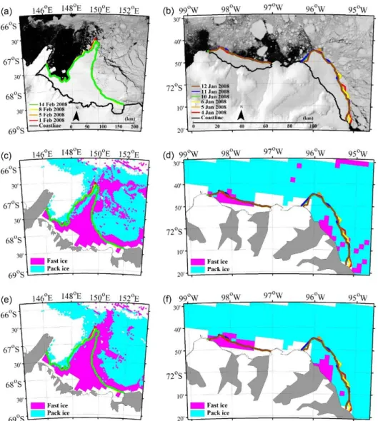
MODIS images with the maximum fast ice cover were used as background images in (a) and (b). MODIS images with the maximum fast ice cover were used as background images in (a) and (b). 26 Figure 2. 8. Temporal variation of fast ice in the Antarctic using a) the simple counting approach and b).
The gray area is Antarctica, and the red and blue solid lines above the sea ice area indicate the fast ice reference edge. The red solid lines indicate the fast ice reference edges marked from SAR images. Time series of fast ice for the ice shelf region, including (a) extent of fast ice and (b) its.
Rapid ice time series for the Sulzberger Ice Shelf site including (a) rapid ice extent and (b).
1
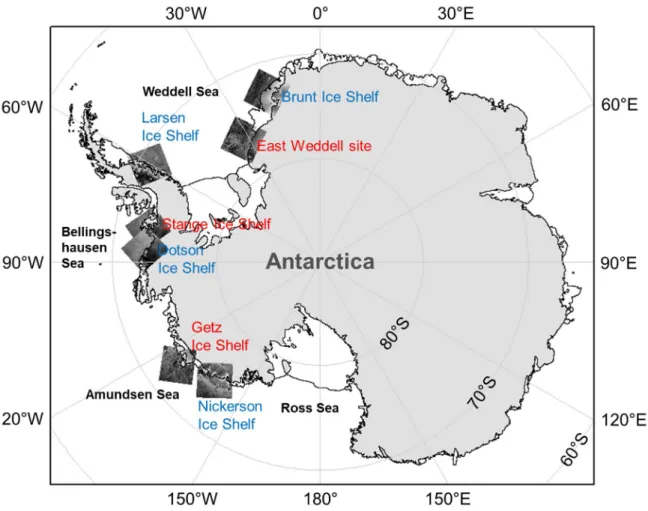
- Importance of the Antarctic sea ice
- Background and importance of landfast sea ice
- Satellite remote sensing of fast ice
- Machine learning techniques for fast ice detection
- Goals of this dissertation
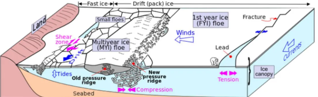
There is no precise standard for the length of time cold ice must be present (Mahoney et al., 2006). For East Antarctic fast ice, it has been created at intervals of 20 days (Fraser et al., 2010). Fast ice forms upwind of the outcrop by advection of packed ice in the wind direction.
Although the extent of solid ice is a relatively small part of the total extent of sea ice, its thickness and volume are. Cloud-free TIR/visible AVHRR imagery was used to investigate the distribution and variations of solid ice along the Adélie coast, East Antarctica (Massom et al. 2009). Another study used only the passive microwave data to develop a model for recording fast ice (Nihashi et al., 2015).
Recently, InSAR approaches have been applied to distinguish fast ice regions (Meyer et al., 2011; Han et al., 2015).
10
- Abstract
- Introduction
- Data
- Methods
- Results and discussion
- Conclusions
The objectives of this study are to (1) develop an automated model based on machine learning approaches for fast ice mapping by synergistically using time series of optical and passive microwave data sets for the entire Antarctic region, (2) investigate patterns of accuracy of time series mapping results, (3 ) examine important variables for fast ice identification by the model and how they affect fast ice mapping results, (4) compare fast ice mapping results with manually extracted fast ice edges from 250-m MODIS images for specific regions of interest, and (5) analyze the spatial- temporal variations of Antarctic fast ice. Because dead ice forms over a wide area attached to shores, the concentration of sea ice in dead ice is about 100%. Spatio-temporal patterns of fast ice distribution were studied using 6-year time series of the produced volume of fast ice.
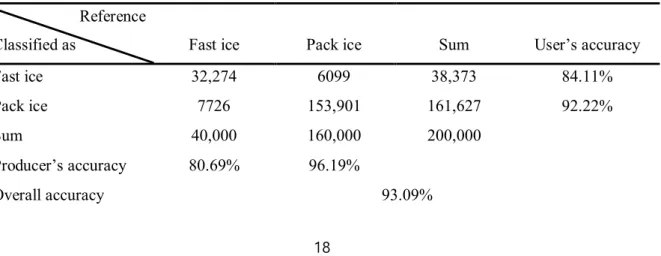
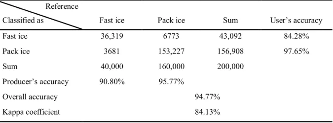
The UA and PA of pack ice were higher than those of fast ice for both models. Ice velocity and IST were the most contributing variables to fast ice classification regardless of the model used. Therefore, the microwave radiation properties, i.e. the brightness temperature, of the ice blocks similar to that of the fast ice (not shown).
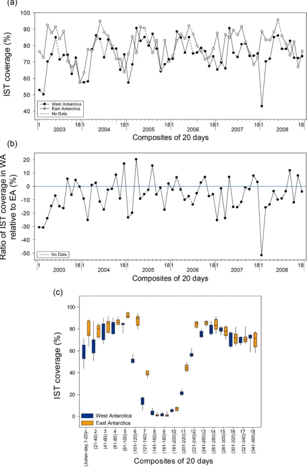
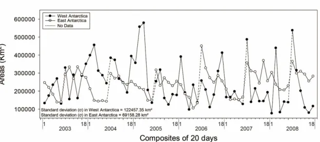
However, significant changes in fast ice areas over 20 days were often observed in East and West Antarctica in MODIS images (Figure 2.4). The limited spatial coverage of the IST could increase the uncertainty of the Antarctic fast ice distribution. A time series of fast ice extent is shown for East and West Antarctica between 2003 and 2008 in Figure 2.
Consequently, the temporal (seasonal and annual) variation of rapid ice dispersal in West Antarctica should merit further research. Ice speed and IST were identified as the most contributing variables to fast ice classification regardless of the approach used. Based on time series of fast ice maps produced by RF, spatiotemporal variations of fast ice were examined across the Antarctic.
The residence time of the dead ice was relatively long in East Antarctica, indicating gradual changes in advance and retreat of the dead ice. However, the residence time in fast ice in West Antarctica was very short, partly due to missing pixels from the MODIS IST data.
28
Abstract
Introduction
Data and Methods
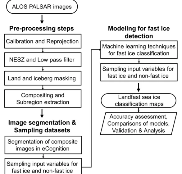
Therefore, by using two consecutive SAR images with a certain time interval, it is possible to define fast ice regions as stable or unchanged ice patches over time. By composing the SAR images at a certain time interval, two consecutive SAR images were used for rapid ice detection through image segmentation and object-based classification. However, in a pair of images with a time gap of several days, the sea ice and open water opacity values are blended into a composite image object segmented according to the presence of sea ice in the nonfast ice regions.
The STD variable can be used to distinguish fast ice from non-fast ice regions. No significant change in the fast ice regions between the two dates allows for more intact spectral values than in the floating pack ice regions. The STD of the posterior distribution values may be increased in pack ice regions due to a wide range of pixel value changes between two dates compared to fast stationary ice regions.
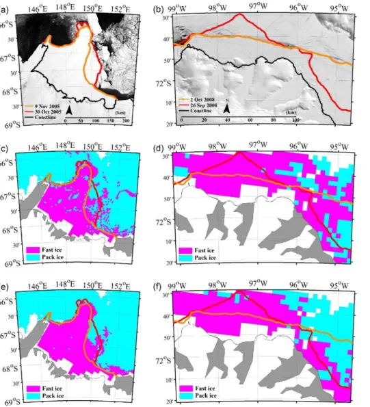
Seaward fast ice edges were determined by distinguishing fast ice and pack ice (i.e., non-fast ice) regions by analyzing the characteristics of surrounding features and changes in backscatter values measured over time (Figure 3. 3 ). Although backscatter varies within fast ice regions, fast ice regions show consistent backscatter values over time compared to pack ice regions. Previous fast ice studies have used MODIS imagery to extract fast ice regions as reference data (Massom et al., 2010; Kim et al., 2015).
Figure 4 shows that SAR and MODIS images are available at a 5-day time interval (31 October 2010 - 5 November 2010) for the fast ice regions on the Getz Ice Sheet over the Amundsen Sea sector to provide quality assurance of the fast ice regions. Although parts of the images are covered by clouds, areas of fast ice are recognizable, bounded by the edge of fast ice (red line) in the MODIS images. Example of 5-day time-lapse SAR images used to detect the fast ice edge for reference over the Amundsen Sea and Bellingshausen Sea sectors.
The machine learning approaches used in this study are RF, ERT and LR for developing fast ice classification models. The classification models were applied to other fast ice regions of interest over the Weddell Sea, the Bellingshausen Sea.
Results and Discussion
On the contrary, small non-fast ice objects near the seaward fast ice edge were misclassified as fast ice due to the stationary backscatter strength of small segments. Fast ice objects located at the edge of seaward fast ice were occasionally misclassified into the non-fast ice class due to the low correlation between two dates. Fast ice detection models were tested for several fast ice areas over the other ocean sectors (Figure 3. 8-12).
A few ice objects were misclassified as solid ice by the ERT and LR models (Figure 3. 8b and Figure 3. 9c). The misclassified fast ice areas show some spatial variation of the surface over time in SAR images. The fastis area on the Nickerson Ice Shelf showed relatively low backscatter, indicating that the ice surface is smooth.
The roughening of the ice surface due to frost flowers occurring in relatively flat regions of fast ice can also increase backscattering (Karvonen, 2004). In the fast ice zone on the Nickerson Ice Shelf, it was confirmed that the surface of objects that were misclassified as non-fast ice changed over time. We note that there is also no apparent influence of incidence angles on the fast ice classification results.
Antarctic sea ice map data were used to evaluate the reliability of fast ice detection models using object-based SAR data. Sea ice map data obtained on 15 November 2010 for the fast ice region in the Bellingshausen Sea were available. There is no fixed time interval appropriate for the delineation of fast ice.
The biweekly Antarctic sea ice chart defined a slightly wider area as fast ice, despite using a longer time interval than this study. The solid blue line is the fast ice edge as a reference. d-f) Results of machine learning models (RF, ERT, LR, respectively) with fast ice edge as reference (solid red line).
Conclusions
51
- Abstract
- Study area
- Data and Methods
- Results and Discussion
- Conclusions and Future Work
MODIS IST data was used as one of the main input data for fast ice detection. As validation data, ALOS PALSAR SAR images were used for quantitative evaluation of fast ice maps. The accuracy of the fast ice reference data was compared with fast ice detection results.
Number of samples for fast ice and non-fast ice class per season and algorithm. The generated fast ice maps were compared with SAR images obtained from ALOS PALSAR data. The corresponding SAR images from ALOS PALSAR show relatively low backscatter over the fast ice region.
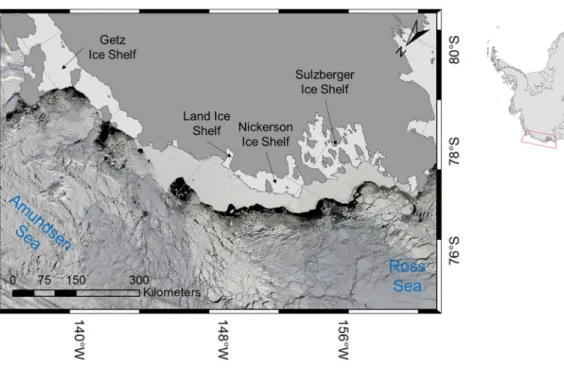
Fast ice is mainly distributed along the coast from the land ice shelf to the Sulzberger ice shelf. Because the bathymetry over the Sulzberger Ice Shelf regions is relatively low, dead ice constantly exists. It was obtained by counting the switches between fast ice and non-fast ice throughout the study period.
The higher values indicate a large variation between fast ice and non-fast ice and vice versa. In Figure 4.7c, the fast ice zone on the Sulzberger ice shelf lasts longer than the land shelf. However, we confirmed that the anomalous fast ice collapse between 2004 and 2005 took place in the ice shelf.
Fast ice time series for the Sulzberger Ice Shelf site, including (a) fast ice extent and (b) its. Spatiotemporal variation of fast ice extent was investigated with particular focus on the Land and Sulzberger ice shelves in the Amundsen Sea.
68
Important role for ocean warming and increased ice sheet melting in Antarctic sea ice expansion. A method for compositing polar MODIS satellite images to remove cloud cover for land-based sea ice detection. Generation of high-resolution East Antarctic land-locked sea-ice maps from cloud-free MODIS satellite imagery.
Seasonal and interannual variations in oceanic heat flux beneath the Antarctic land ice sheet. Sea ice motion from satellite passive microwave imagery estimated by ERS SAR and buoy motion. The new visualizations highlight new information about contrasting Arctic and Antarctic sea ice trends since the late 1970s.
Conditions leading to the record low Antarctic sea ice extent during the 2016 austral spring season. Structure, salinity and isotopic composition of perennial land-locked sea ice in Nella Fjord, Antarctica. Polarimetric properties of sea ice in the Sea of Okhotsk observed by airborne L-band SAR.