Development of three-dimensional parallel code to study the motions of particles in a fluid using. The code is the combination of the two models, the Shan-Chan multiphase model for a viscous fluid, the pseudo-solid model for particles. This code can be used to simulate the dynamics of self-assembly driven by evaporation and any multiphase flow with different sizes of particles.
Introduction
The latest improvement and theoretical basis of the three models are well organized in Huang's recent work [17]. Calculation in LBM is local, so the LBM model can efficiently calculate the interaction between fluid and particles. Above all, the advantage of LBM, the scalability on parallel computers, is undoubtedly the primary reason for the increasing interest in LBM.
DASSAULT SYSTEMS takes over PowerFLOW, which was the first commercial software based on LBM, in 2017. NUMECA is merged with Palabos in 2018, which has been the most popular and versatile open source software in LBM community. Although developing in-house code in a laboratory may seem like an impractical task when reliable and powerful software already exists, the LBM are still new methods that require extensive improvements.
The internal codes will help those who want to develop or adopt them for their own problems. Moreover, a simple internal code is easy to read without in-depth knowledge of programming technique and useful to understand the basics about the method.
Simulation methods
Lattice Boltzmann Equation
One macrostate corresponds to a multitude of microstates, so we can simply choose the most manageable one. Moreover, the collisions tend to dissipate the momentum of each particle and after a sufficient number of collisions the system settles into an equilibrium state. Therefore, the time rate of change of the distribution function is proportional to how far the drop deviates from equilibrium and inversely proportional to the time between collisions.
The actual discretization process requires some mathematical background on Hermitian series expansion and is beyond the scope of this paper. The normalized grid spacing Δ𝑥 and time step Δ𝑡 are usually set to 1 grid unit for simplicity. The LBM simulation and the real system can be compared using dimensionless numbers such as Reynolds number, Bond number and capillary number.
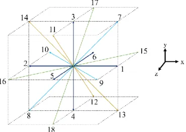
Hence, 𝜏 is equal to Δ𝑡, which means the system is in equilibrium at each time step because relaxation time is equal to time step. They are classified using notation DdQq, where d is the number of dimensions and q is the number of discretized velocities.
Shan-Chan Two Component Model
Without the interaction force between the two liquid components, this system can be considered as an ideal gas mixture and has some common equilibrium velocity, 𝐮𝑒𝑞[11].
Particle Model
- Particle domain
- Particle-fluid interaction
- Particle-particle interaction
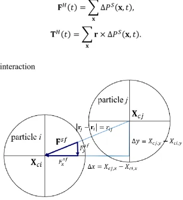
At each grid point in a fixed particle, the local velocity of a particle component is determined by the particle's translational velocity and angular velocity. The common velocity of the SC model at each point can be found by taking into account the effect of the particle component. Hydrodynamic force on the particle of each component of fluid is determined by calculating momentum change of fluid at each node.
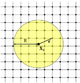
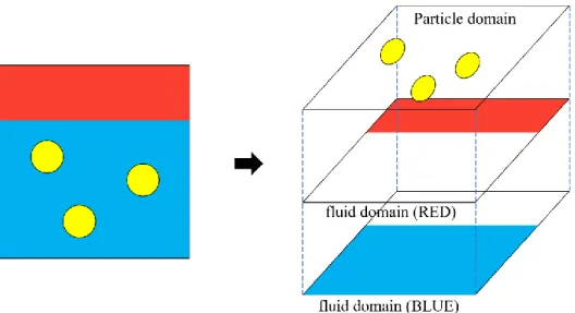
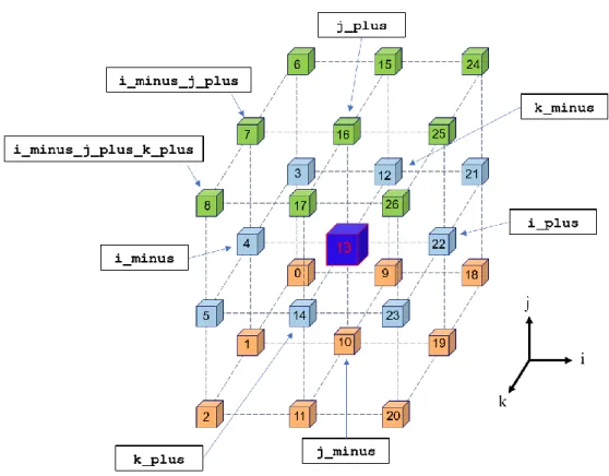
The total hydrodynamic force on the solid particle can be obtained by collecting in the particle domain the grid points where 𝑛𝑃(𝐱) ≠ 0. For particle simulation, each of the 26 neighboring processors must be known to appropriately handle the particles that span more than two processors. For the particle model, another domain layer named particle_domain is added to the two fluidRED and fluidBLU layers.
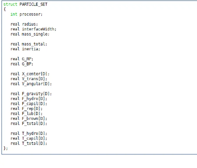
Once the particle density is calculated for all points on the particle domain, it behaves like any other SC fluid component, retaining its shape. To set the particle density on the particle domain, the information in the PARTICLE_SET structure is used. If the particle has no effect on it, it returns -2, and if the particle belongs to it, it returns -1.
It can then be used to set the particle domain to its domain in the usual way. For example, if the particle rotates about a stationary axis, the local velocity field looks like Fig. Although its translational velocity is zero, the local velocity cannot be zero if the particle has an angular velocity.
After the force is calculated with PARTICLE::calc_force_single(), the partial forces distributed over multiple processors must be collected into the processor responsible for the particle using PARTICLE::MPI_reduce_force(). For example, to get the corresponding force value per particle in the image. If the updated position is outside the local domain area, it means that the particle moves to the neighboring processor. After that, the neighboring processor becomes responsible for that particle and the processor should know that it is a particle.
Details of the Program
Velocity Set
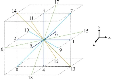
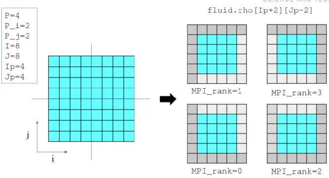
Domain Decomposition
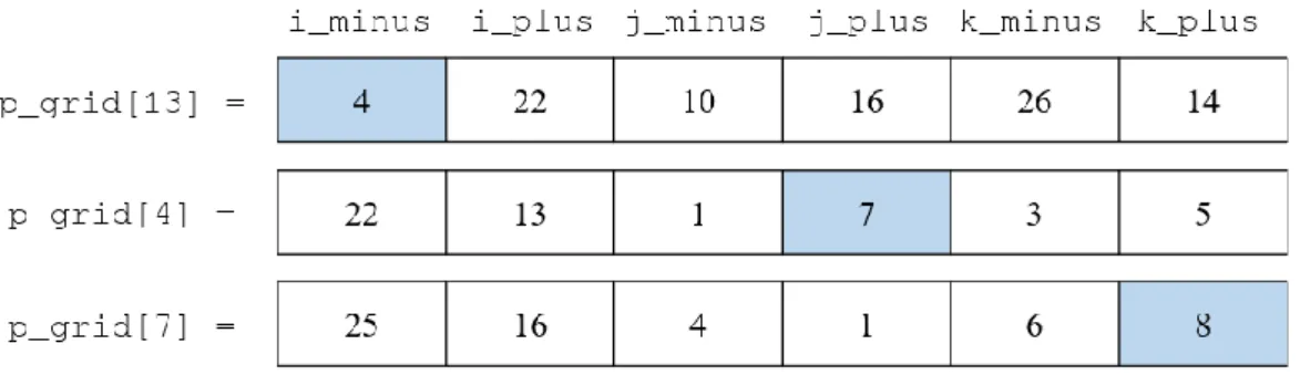
The names for other processors can be found in the first few lines of src/particle.cpp. A boundary condition must be applied to a boundary node outside the computational domain and a proper distribution function must be provided. The effect of the external force is included in the equilibrium velocity with the SC forcing scheme.
After determining the density and velocity of the fluid, the distribution function must be determined. First, the boundary conditions can be applied directly to the missing distribution function at the outermost part of the computational domain. According to the applied boundary condition, the missing distribution function will be assigned the correct value.
The effect of angular velocity along other axes can be calculated in a similar way. The lattice Boltzmann methods are a relatively new method, but several models have been proposed to handle the dynamics of particles in a viscous fluid, which are consistent with the conventional methods. The pseudo-solid model is one of the latest Boltzmann lattice methods for colloidal particles.
Luo, Theory of the lattice Boltzmann method: From the Boltzmann equation to the lattice Boltzmann equation, Phys. Chen, Simulation of non-ideal gases and liquid-gas phase transitions by the lattice Boltzmann equation, Phys. Chan, Simulation of multicomponent fluids in complex three-dimensional geometries by the lattice Boltzmann method, Phys.
FLUID Datatype
Neighboring Processors
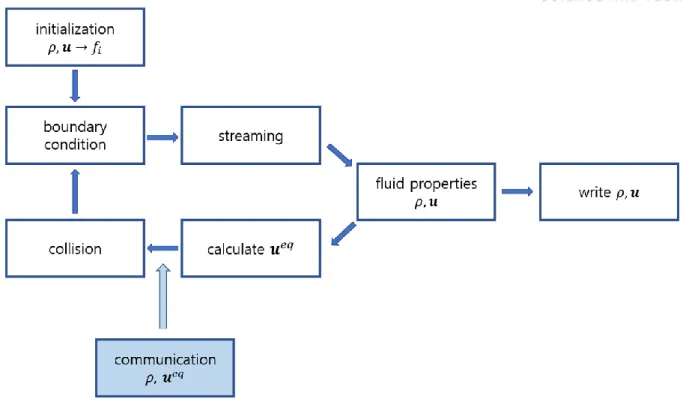
Sequence of Substeps
After it is initialized, the main loop can start with collision or current, or the application of boundary condition. Although this does not affect the result, one must be aware of it when writing code for initialization or boundary condition. With the sequence of substeps shown in fig 00, initialization must specify the distribution function as well as the fluid properties.
If the loop starts with a collision, there is no need to calculate the distribution function for initialization, and if the boundary condition is applied after the streaming process, no additional boundary nodes are needed. Using the updated distribution function, the fluid properties are calculated and stored based on the write frequency values.
Initialization
However, there are an infinite number of possibilities because an infinite number of microstates correspond to a macrostate.
Boundary Conditions
Communications
Since the data to be passed on the boundary is not continuously stored in memory, we need to package the data to be sent into an array and create an array to store the incoming message. The continuous data on the temporary array is written to the appropriate border node on the local array.
Two Component Model
Particle Model
- Density
- Local velocity
- Force gathering
- Position update
When more than two processors are used for a simulation, it is possible for a particle to span over the neighboring processors, as described in Fig. If so, it returns the processors' relative position with respect to it using the naming convention shown in Fig. Using the return value of find_neighbor() and the particle position in the local domain of that processor, calc_X_center() adjusts the position.
When the position of the particles is as in Figure 22, the resulting particle_domain.density[Ip][Jp] looks like Figure 26 describes how to include the effect of angular velocity in local velocity calculations. However, when a particle spans more than two processors, each processor computes only a portion of the power, as described in Figure 27.
Different contact angles can be simulated with the SC model by adjusting the strength of the interaction force between the fluid and the wall. The initial state is the rectangular shape of the first liquid component surrounded by the other liquid component. The method is installed in this code, so many experiments and numerical validations can be performed with this code to improve the model.
The code also takes into account the parallel computation, which is one of the main advantages compared to the conventional methods of computational fluid dynamics. This code is carefully verified in the simple examples to avoid the unphysical behavior of particle motion and thus can be further extended to study more complex problems.
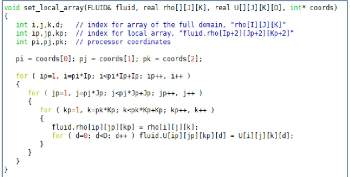
![Figure 13. rho_init[I][J] and the local array.](https://thumb-ap.123doks.com/thumbv2/123dokinfo/10509731.0/27.892.107.788.769.1074/figure-13-rho-init-and-the-local-array.webp)
