This paper proposes long-term displacement measurement methods using computer vision and LiDAR, adapted for full-scale bridge structures. The computer vision-based approach compensates for errors caused by camera movement using an auxiliary camera, and long-term displacement can be achieved independently of camera movement.
Introduction
Motivation and Scope of the Research
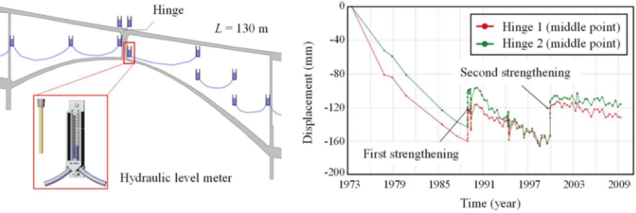
On the other hand, long-term movement monitoring is a challenge for large-scale bridges. LiDAR-based method can measure long-term displacement without permanent installation of the sensor in the field, so no drift error is expected.
Dissertation Overview
Literature Review on Displacement Measurement Methods
Displacement Measurement Methods
- Indirect displacement estimation approaches
- Direct displacement measurement approach
Denoting y as the location of the strain gauge relative to the neutral axis, the curvature can be calculated by dividing y by the strain. Although sensors in Category 1 provide sub-mm displacement resolution, physical contact of the sensor with the bridge is generally impractical for field applications.
Limitation of the Displacement Measurement Methods in Long-Term Monitoring
- Existing field applications of the long-term displacement measurement
- Limitation of computer vision and LiDAR-based approaches in long-term application
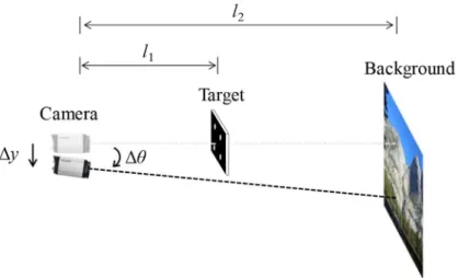
When a camera is installed for long-term monitoring of an entire structure, unexpected camera movements are inevitable. Conventional computer vision-based displacement measurements have problems with applicability to the long-term measurement of entire civil structures.
Summary and Discussion
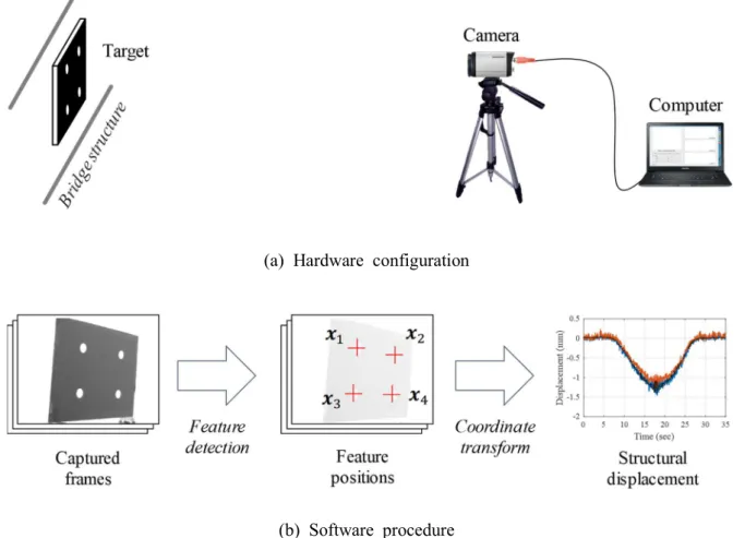
Vision-Based Long-Term Displacement Measurement System
Introduction of dual-camera system
Long-Term Displacement Measurement based on Dual-Camera System
- Basic camera geometry involved in the proposed method
- Formulation for true displacement
- Formulation of frame-invariance transform matrix with main camera
- Formulation of camera motion-induced error with sub-camera
- Displacement calculation with the error compensation
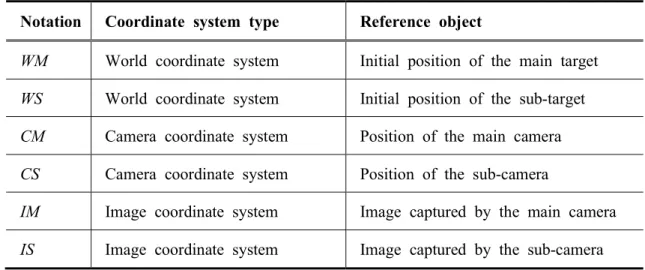
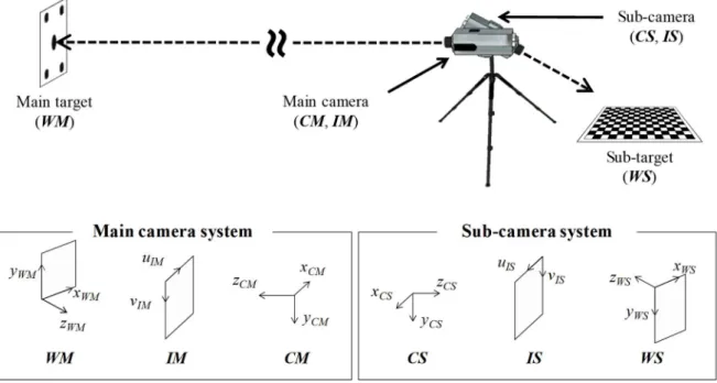
WM and WS are the world coordinate systems defined by the starting positions of the main and subtargets, respectively. CM and CS are the camera coordinate systems defined by the main and sub camera positions, respectively. IM and IS are the image coordinate systems for the main and sub cameras, respectively.
However, this study includes any combination of j and k to express the position of the main target in terms of constant camera position. As shown in this example, two different time indices effectively indicate the position of the main target in any given camera position. If the main camera is affine, the third row of the transformation matrix BWM → IM(k) in Eq.
Thus, the 6-DOF motion of the sub-camera relative to the initial position is expressed as BCS(1)→CS(k). As discussed for Eq.(3.8), the spurious displacement at the k-th frame is the starting position of the main target represented in IM(k), which is Eq. The main camera measures {ui(k) vi(k)}TIM(k) for each feature point in the kth frame of the main target.
Validation
- Numerical validation
- Laboratory-scale validation
Because the main target was fixed, the displacement measured by the main camera without error compensation was the false displacement due to camera movement, as shown in Figure 22(a) . Two industrial-grade cameras were rigidly attached to each other from steel plates to construct the dual cameras. Pan-tilt was installed under the dual cameras (see Figure 23) and used for camera calibration to determine the unknown parameters in Eqs.
After calibration, the pan-tilt motor was manipulated to generate gradual three-dimensional rotations and translations of the dual cameras to simulate prolonged camera movements. The dual-camera system has been carefully designed to meet the long-term displacement measurement assumptions outlined in Section 3.2. Therefore, the assumptions that motions other than that of the dual camera are fixed were valid for the laboratory-scale experiment. a) Composition of the dual camera.
The displacement measured by the main camera without error compensation (referred to as "single camera" hereafter) was compared with that corrected by the dual camera system. The spurious displacement was compensated for with the dual camera system, resulting in a spurious displacement of 1.1 mm as shown in Figure 26(b). 6-DOF camera movements for the lab test. a) Comparison between the dual-camera and single-camera methods.
Summary and Discussion
LiDAR-Based Long-Term Displacement Measurement System
- Introduction of the LiDAR-based displacement measurement system
- Long-Term Measurement based on Strategic Reflector Topology
- Reflector topology
- LiDAR-based displacement computation algorithm for long-term monitoring
- Validation
- Laboratory-scale validation
- Summary and Discussion
The proposed method uses reflectors attached to specific locations on the outside of the bridge to be measured. The reference vector, {s}k, at the k-th measurement is defined as an average of the 3D coordinates for each reflector in the reference group axis. LiDAR measures the varying positions of the reflectors in the measurement group over time, and these measurements are then used to calculate displacements relative to the reference vector.
The proposed method provides a scanning scheme that efficiently determines the reflector positions with minimal manual handling of the point cloud. Vertical deflection of the bridge deck is calculated as the vertical component of the {pi}k for the ith point at the kth measurement. Therefore, the vertical displacement of the i-point at the k-th measurement with respect to the initial measurement can be written as. 4.6) The formulation for the vertical displacement is independent of all different LiDAR positions at each measurement.
Displacements were measured using three different LiDAR positions to investigate the LiDAR position independence of the proposed method. For each measurement location, static loads were increasingly applied to the center of the desk. The position of the reflectors is used to calculate the long-term displacement, comparing the deviation from the initial measurement in the vertical direction.

Field Validation of Proposed Displacement Measurement Systems
Experimental Setup
- Testbed information
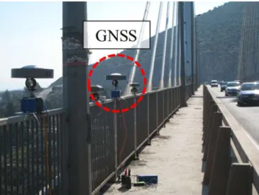
- Sensor deployment scheme
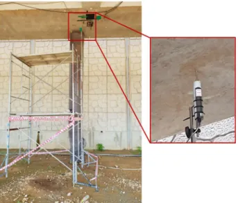
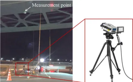
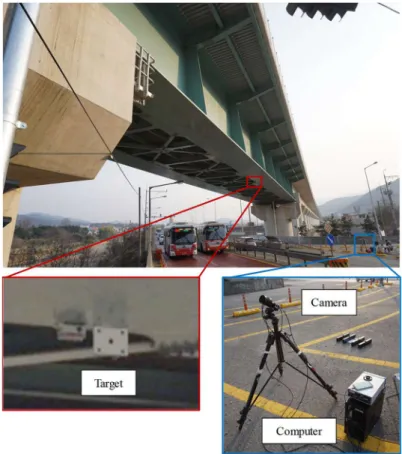
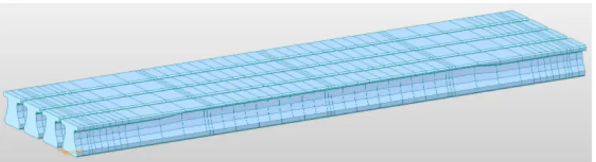
A finite element model of the target bridge was implemented to simulate long-term displacement. A dual camera system was installed on the pier to measure the movement of the main target attached to the mid-span for 548 days without occupying the space under the bridge. Note that the LiDAR was acquired after each measurement, thus avoiding permanent installation of the sensor in the field.
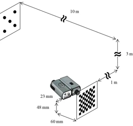
Due to pressure under the bridge in September 2018, these contact sensors stopped measuring 72 days after installation. The main target was attached to the center of the bridge with five white circles and a black background. Due to the light weight of the target and strong adhesion, it was intended that the sub-target is permanently attached to the pier without movement.
The LiDAR system was regularly installed in the field to measure the long-term mid-bridge displacement relative to the stationary piers. The location of the reflectors on the deck and piers was measured by the temporarily installed LiDAR as shown in Figure 38(b). To contact the tip of the LVDT with the bridge, a scaffold was placed under the bridge that allowed the measurement of the displacement relative to the ground.
Field Test Result
- Long-term displacement analysis
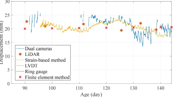
For the first 5 days of displacement measured with dual cameras, 5 mm of daily displacement due to sunlight was observed during the day. Snow accumulated on the slab at the age of 148-151 days, while the impact of snow was negligible. In addition to weather conditions, swarming of insects in front of the camera lens and objective, as shown in Figure 60, resulted in the error for dual cameras at 223, 228, 233, and 234 days of age.
No additional load was applied until the age of 333 days. For the first stage of ballast placement, 1.6 mm, 3.0 mm, 2.0 mm, 2.5 mm and 2.4 mm of instantaneous displacement were measured by means of dual cameras, LiDAR, strain-based method, LVDT and ring gauge respectively. In the same order of the sensors, 0.9 mm, 2.0 mm, 1.6 mm, 1.6 mm and 2.0 mm of the instantaneous displacement were respectively measured for the second phase of the ballast placement.
In the case of LiDAR, a cable tie near a reflector, as shown in Figure 53(a) , caused measurement errors on the 333rd and 356th day. Similarly, −0.2 mm and 0.0 mm high displacement were measured by the dual cameras and LiDAR around a summer solstice on the 644th day. On the other hand, the strain gauge stopped its operation due to the accumulation of the drift error.
Performance of the proposed long-term displacement measurement methods
- Discussion on vision-based long-term displacement measurement
- Discussion on LiDAR-based long-term displacement measurement
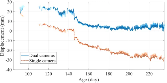
The camera movements resulted in the drift error shown in Figure 58, where the single camera (ie, main camera only) measured a displacement 30 mm greater than that measured by the dual cameras. The spurious displacement was even larger than the true structural displacement, clearly showing why the camera motion-induced error must be removed for reliable long-term measurement. The dual-camera system was demonstrated to accurately measure the long-term structural displacement by compensating for the error due to camera movement.
The 3D positions of the reflectors can be estimated quickly and reliably using targeted scanning and binarization-based segmentation. Given that the minimum number of points covered by one reflector is 1,000, the standard deviation of the distance scan is expected to decrease from 5 mm for a single point to 0.16 mm for the centroid when the central limit theorem is considered [154]. The use of a 3D point cloud of the entire bridge turned out to be unsuitable for measuring bridge displacements.
The position data of the following two lines were manually extracted from the scanned point cloud: the southern line with points b1, b3 and b5 and the northern line with points b2, b4 and b6, as shown in Figure 38(a). By averaging the vertical components of the point cloud position data for each 2.5 m interval, the vertical positions along the longitudinal axis of the bridge were obtained as shown in Figure 60. The resulting standard deviations of approximately 5 mm are shown as the I-shaped bars in Figure 60; this value is unacceptably large for measuring the displacement of short and medium span bridges.
Summary and Discussion
Conclusions
Jang, S., et al., Structural health monitoring of a cable-stayed bridge using smart sensor technology: Introduction and evaluation. Cho, S., et al., Structural health monitoring of a cable-stayed bridge using wireless smart sensor technology: data analyses. Bocca, M., et al., Synchronized wireless sensor network for experimental modal analysis in structural health monitoring.
Tennyson, R., et al., Structural health monitoring of innovative bridges in Canada using fiber optic sensors. Lee, J.J., et al., Development and application of a vision-based displacement measurement system for structural health monitoring of civil structures. Fu, T.S., et al., Energy-efficient implementation strategies in structural health monitoring using wireless sensor networks.
He, C., et al., A combined optimal sensor placement strategy for structural health monitoring of bridge structures. Park, S., et al., Multiple crack detection of concrete structures using impedance-based structural health monitoring techniques. Dworakowski, Z., et al., Vision-based algorithms for damage detection and localization in structural health monitoring.