The CDFs evolve over time due to the randomness of media interfaces. With singular perturbation analysis, we can derive the so-called correctors, which are analytical approximations of the rigid parts in the solutions.
Theory of Nonlinear Hyperbolic Conservation Laws
Characteristics Method
The cutoff time t∗ at which collision occurs can be determined using the implicit function theorem (see e.g. [26]) for Eq. Therefore, we look for a weaker sense in which we can define solutions, which are called weak solutions.
Integral (Weak) Solutions and Their Properties
Then if u is a weak solution of Eq. 2.1.1), it satisfies the following jump condition. where [g] = gL−gR indicates the jump of g over the curve C. s is called the propagation speed of the discontinuity. A smooth function U(u) is said to be an entropy function if it satisfies the following conditions:
Characteristic Decomposition
Monotonicity preserving property means that no new local maximum or minimum is created in the solution of the conservation law, and the maximum (minimum) values do not increase (decrease) as the solution evolves in time. Note that system (2.1.29) is now decoupled and each characteristic component wk(x, t) can be solved exactly.
Numerical Methods for Conservation Laws
Notations
Conservative Methods
A conservative method has the following form. where the numerical flux ˆ fj+1. in accordance with the analytical flux, i.e. 2.2.9) The advantage of a conservative method is shown in the Lax-Wendroff theorem below which shows the convergence to some weak solution of Eq. Lax.
Total Variation Stability, Convergence, and Discrete Entropy Condition . 17
The uniform bound in space with respect to total variation implies a uniform bound in time, as appears from the following lemma (see [96]). In the following sections, we mention commonly discussed TVD schemes, starting from the first-order ones.
First-order Schemes
- Godonov’s Scheme
- Other Schemes
The Godonov scheme, due to exactly solving a Riemann problem to approximate. Roe's scheme is especially efficient for a system case, for example the Euler equations ([118]), due to its simplicity.
High-resolution TVD Schemes
- Flux-limiting Schemes
- Slope-limiting Schemes
To satisfy the TVD condition (2.3.5) which prevents the generation of oscillations, we need to limit the slope γj in some sense. In fact, comparing (2.3.5) and the TV stability condition (2.2.26), the uniform constant M is not necessarily the TV of the initial data.
Essentially Non-Oscillatory (ENO) Schemes
- Semi-discrete Discretization
- Reconstruction
- Numerical Flux
- Characteristic Projection
Let rt and rx be the orders of precision of the time integrator and the spatial discretization, respectively. The softness of the solution in each cliché is determined by a softness indicator.
Overview
- Finite Difference Schemes
- Time Integration
- Reconstruction
- WENO-JS
- Mapped WENO
- WENO-Z
- Reconstruction
- WENO-NW6
- WENO-CU6
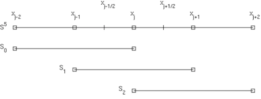
¯ hj is called an average value of the numerical flux h(x) over the interval Ij. A treatment is needed in the more upwind S3 sub-stencil to support the ENO property of the scheme. The differences lie in the softness index of the windiest β3 sub-stencil and that of the large S6 template.
The smoothness indicator of the large stencil S6 is defined as the highest, that is, fifth degree, undivided difference as follows.
The New 6th-order WENO-θ Scheme
- An illustrative example
- The New Scheme
- Central Reconstruction, New Central Smoothness Indicators ˜ β k
- New τ θ
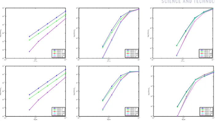
- Accuracy Tests
- Resolution Tests
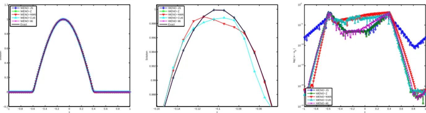
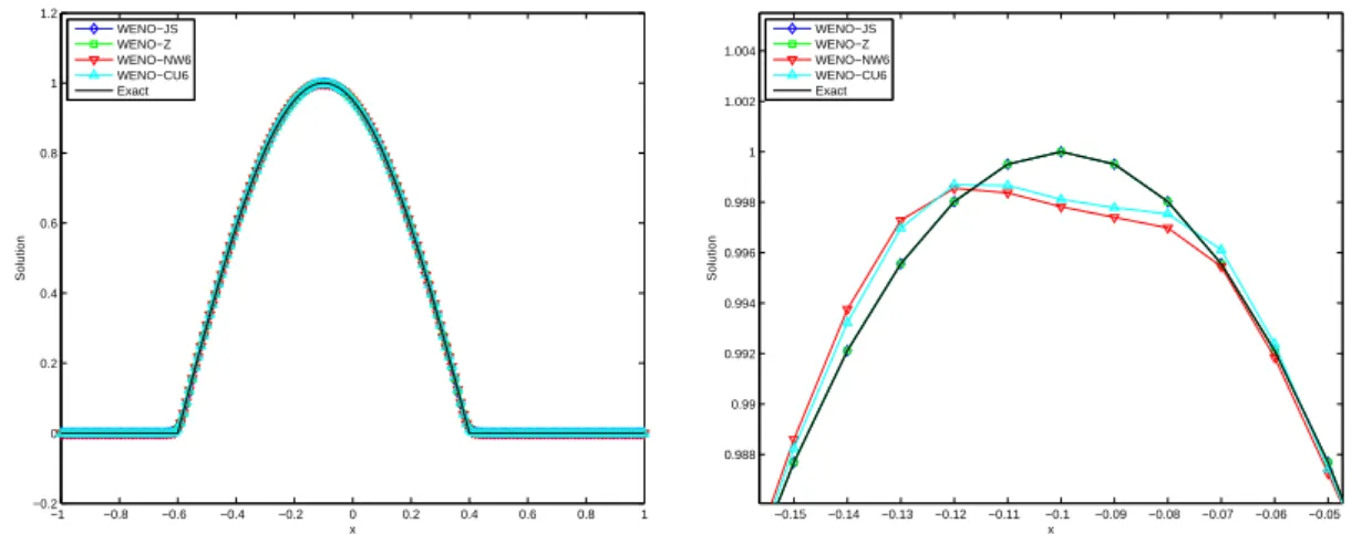
- TEST 1: Linear Case
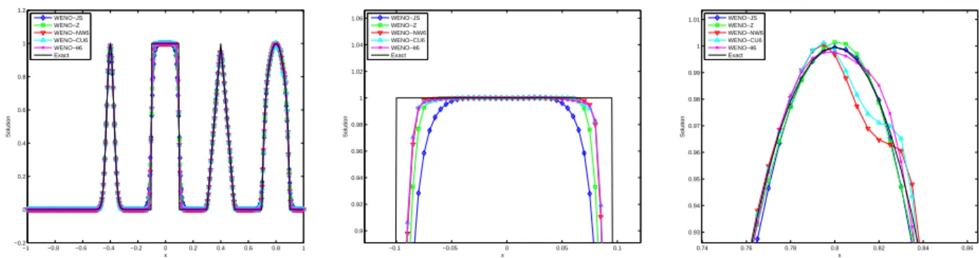
- TEST 2: Nonlinear Case
The above defect of WENO-NW6 and WENO-CU6 schemes is clearly shown. The scheme is therefore 5th order upwind or 6th order central depending on the smoothness of the S5 and S6 templates. We also notice the non-convergence of the ωk of the WENO-CU6 and WENO-NW6 schemes around the critical region.
4-2 we show the numerical results of the 6th order WENO schemes for the initial state.
Euler Equations of Gas Dynamics
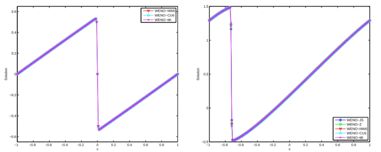
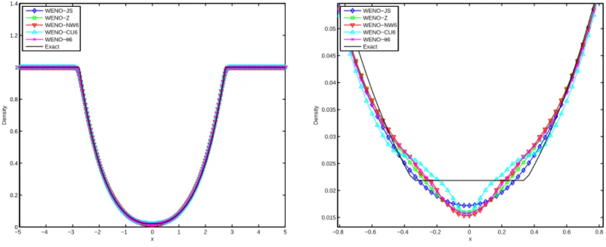
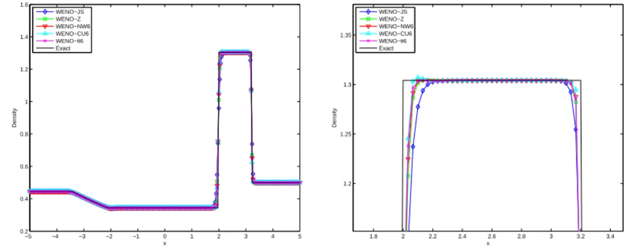
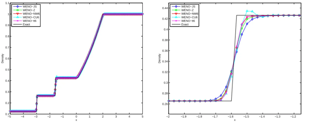
TEST 3: Riemann Problems
Numerical results of the density obtained from all WENO schemes with a grid of N = 300 are shown in Fig. It is shown that WENO-NW6 and WENO-θ6 have the sharpest capture of the discontinuities for the Sod problem. For the Lax problem, we note an overshoot at the contact discontinuity around x = 2 of the WENO-NW6 and WENO-Z schemes; whereas the WENO-θ6 does not experience this.
It is also observed that for problem 123, WENO-JS, WENO-Z and WENO-θ6 are better than WENO-NW6, WENO-CU6 in approximating the trivial contact discontinuity aroundx=0.
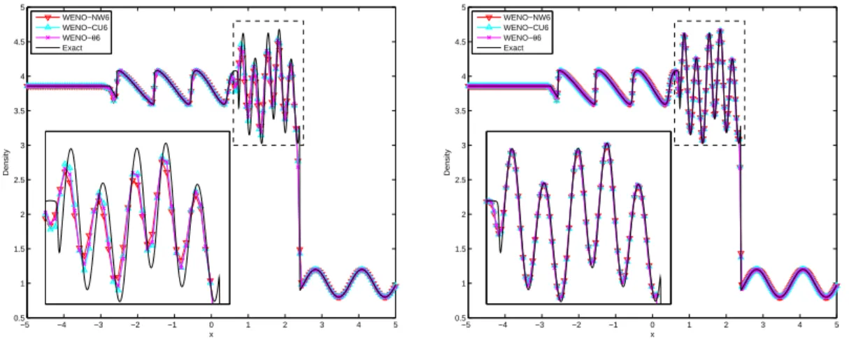
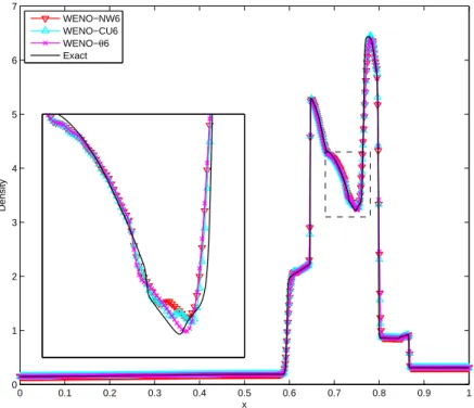
TEST 4: Shock Density Wave Interaction
TEST 5: Two Interacting Blast Waves
This problem is used to test the robustness of impact capture methods as many interactions are observed in a small area. We also emphasize that in the solutions of the latter methods in this region there is a phenomenon of a stepped case, which is similar to the one at the top of the semiellipse in test 1 (see fig.
Two-dimensional Euler’s Equations
- TEST 6: Rayleigh-Taylor Instability
- TEST 7: Implosion problem
- TEST 8: 2D Riemann Initial Data
- TEST 9: Double Mach Reflection of a Strong Shock
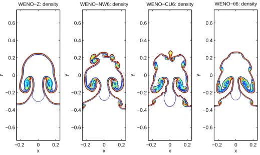
We note that WENO-θ6 preserves the symmetry of the solution; while WENO-NW6 and WENO-CU6 do not. Only WENO-Z and WENO-θ are shown to preserve the symmetry of the problem well; while other 6th order schemes do not. Again, we observe the superior performance of WENO-θ6 compared to the WENO-NW6 and WENO-CU6 schemes over these small-scale structures without contour oscillations.
Numerical results of the density obtained from the 5th order WENO-Z, 6th order WENO-NW6, WENO-CU6 and WENO-θ6 schemes at time = 0.2 are plotted in Fig.
Introduction
The latter method depends on a fairly large number of samples to obtain results; while for PCE methods, the solutions are projected into a random space spanned by orthogonal polynomials whose arguments are the random variables and are equipped with an inner product. In our problems, we choose shifted Legendre polynomials for the random variablesξi following a uniform distribution. If the number of random variables increases, the computational cost will increase exponentially as shown in the polynomial chaos (PC) expansions below, as the polynomials belonging to each random variable are multiplied in a tensor product form.
The number of unknown coefficients (PC modes) therefore grows exponentially and the calculations are very expensive.
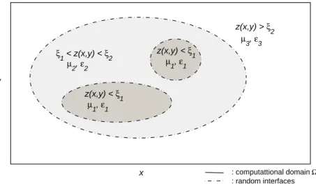
PCE Methods for Multiple Random Interfaces
Case 1
To calculate the solutions of the system (5.2.6), we use the finite difference time domain method (FDTD) according to K. The central finite difference of the 2nd order is used on the offset grid for the spatial discretization of the magnetic and electric fields. On this distributed grid, the magnetic and electric fields are at the sides and center of each grid cell, respectively. The time derivatives are approximated in the same way: the magnetic fields are first updated to a half time step; then the electric field moves to the next time step based on the updated values.
5.2.6), we use the following notations for the magnetic fields H1,2 and electric field E3 at the nodal points on the staggered grid as in Fig.
Case 2
In the following part, we introduce a modification in deriving the PC states which overcomes the drawback discussed above. The entries (ckλkl)1,2 correspond to the coefficients cµik defined in (5.2.5b), respectively with the removal of δik anda, b replaced by appropriatea1, b1 and a2, b2. It is noted that in the system (5.2.16) we treat the matrices H1,E3 as vectors by fixing one index and marching the other.
The PDFs are respectively fi(ξi) =b 1. Note here that although we consider then tensor product of one-dimensional PC expansions, only an integration in one dimension needs to be calculated to find the coefficients in Eq. 5.2.20) and this makes the entire computational cost grow linearly.
Statistics
Numerical Results
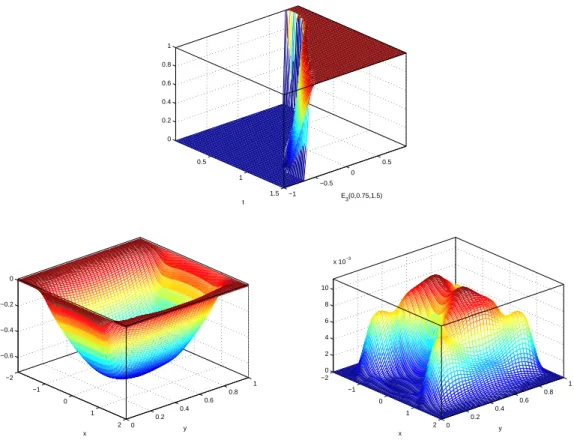
We observe the CDF of the Maxwellian solutions evolving in time for both cases, as shown in the figure. It is shown that the variation of CDF for E3 for the latter case is much wider than the former. Next, the time evolution of the electric field E3 is simulated for the case of 2 compatible initial and boundary conditions, and the results are shown in Fig.
We also check the decay of the PC modes of E3 for both cases of initial/boundary conditions (5.4.2).
Parallel Computing
In the first stage, i.e. the Yee scheme, for parallel purposes we apply the so-called decomposition of the domain in the x-direction to the 2D grid of the computational domain. And in the second case, we test with three random interfaces with initial and boundary conditions (5.4.2) and (5.4.3), aiming to save computational time. 5-11 we plot the computation time (in minutes) for different number of processes used in parallel computation.
A very small time step should be chosen to handle the sharp transition in solid layers.
New Semi-analytical Time Differencing Methods for Stiff ODEs
Classical IF and ETD Methods
- Integrating Factor Methods
- Exponential Time Differencing Methods
Instead of applying the RK time integration directly as in the IF methods, Cox and Matthews ([22]) in their paper suggest an alternative by interpolating the nonlinear term F. That is, instead of a direct calculation of g(z) in Eq. 6.2.11), one can evaluate the function via an integral over a contour Γ as follows. Then a typical quadrature method, for example the trapezoidal rule, can be applied to evaluate the integral numerically.
In casez is real, by choosing Γ as a circle centered atz on the real axis, the computational cost can be reduced by Eq. 6.2.12) with equally spaced points on the upper half of the contour Γ.
The Schemes with Correctors
- Asymptotic Expansions
- The IFRK and ETDRK Schemes with Correctors
In [90], the authors point out that the ETDRK methods are not numerically stable, due to the presence of the term. Since the conventional numerical schemes are now applied for the non-stiff part v=u−θ≈us, it is expected that the results are much improved compared to the same schemes applied directly to the solution u. In [22] (see also [101]), it is pointed out that for a dissipative equation (i.e. ε is real and positive), the solution is attracted to the slow partus, and this can be expressed as an asymptotic expansion of ε as follows.
For the purpose of numerical implementation, since in the combination θ0+εθ1 the last term in (6.2.35) which is multiplied by ε is softer than θ0, by removing the soft term we determine the corrections, θ0, θ1,.
Application to Spectral Methods for the Dispersive KdV Equation
Derivation of the Correctors
Here θbis is derived as below and it turns out that θb captures the stiffness of bu and thus bv becomes mild and slow. Changing time back to t and dropping small nonlinear terms of order O(ε(l)ε(k−l)) on the right-hand side of Eq.
Approximating θ b 1
New Schemes with Correctors
Numerical Results
Stiff ODEs
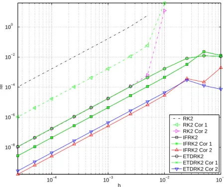
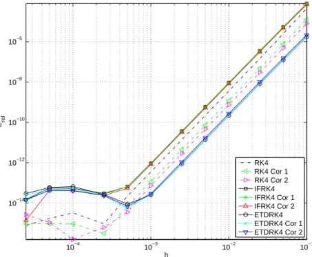
The relative numerical errors of this example are plotted in logarithmic scales in the figure. In numerical simulations, if only θ0 is used as a corrector, the new schemes are similar to the classic IFRK and ETDRK, i.e. to those without correctors. Differences in scheme errors are listed in Table 6-1 for 2nd and 4th order schemes.
For ε = 0.25 with time = 1, in 2nd order schemes ETDRK2 withCor2 outperforms the others as in fig.
The KdV Equation
For the first part of the thesis, we established a new WENO-θ scheme for conservation laws. As a result, the stiffness of the problem is then solved or recorded by the correctors. Here, due to the stiffness of the initial data, they need many Fourier modes in the spectral representations, i.e.
This incurs significant computational costs to obtain the explicit forms of the correctorsθb1(k) due to the modal.