저작자표시-비영리-변경금지 2.0 대한민국 이용자는 아래의 조건을 따르는 경우에 한하여 자유롭게
l 이 저작물을 복제, 배포, 전송, 전시, 공연 및 방송할 수 있습니다. 다음과 같은 조건을 따라야 합니다:
l 귀하는, 이 저작물의 재이용이나 배포의 경우, 이 저작물에 적용된 이용허락조건 을 명확하게 나타내어야 합니다.
l 저작권자로부터 별도의 허가를 받으면 이러한 조건들은 적용되지 않습니다.
저작권법에 따른 이용자의 권리는 위의 내용에 의하여 영향을 받지 않습니다. 이것은 이용허락규약(Legal Code)을 이해하기 쉽게 요약한 것입니다.
Disclaimer
저작자표시. 귀하는 원저작자를 표시하여야 합니다.
비영리. 귀하는 이 저작물을 영리 목적으로 이용할 수 없습니다.
변경금지. 귀하는 이 저작물을 개작, 변형 또는 가공할 수 없습니다.
Toric Hirzebruch-Riemann-Roch
(토릭 힐체브루흐-리만-로흐)
2018년 8월
서울대학교 대학원 수 리 과 학 부
이 재 황
(토릭 힐체브루흐-리만-로흐)
지도교수 Atanas Iliev
이 논문을 이학석사 학위논문으로 제출함
2018년 4월
서울대학교 대학원 수 리 과 학 부
이 재 황
이재황의 이학석사 학위논문을 인준함
2018년 6월
위 원 장 인
부 위 원 장 인
위 원 인
by
Lee, Jae Hwang
A DISSERTATION
Submitted to the faculty of the Graduate School in partial fulfillment of the requirements
for the degree Master of Science in the Department of Mathematics
Seoul National University August 2018
Abstract
In this thesis, our main goal is the Hirzebruch-Riemann-Roch theorem for smooth complete toric varieties. To do this, we start from affine toric varieties and how to con- struct them. Also, projective and abstract toric varieties will be introduced, including their fans and the orbit-correspondence. Next, we briefly explore divisors, line bundles, and cohomology for toric varieties. Finally, after working the equivariant version of the Hirzebruch-Riemann-Roch, using Brion’s equality and taking the nonequivariant limit, we prove the Hirzebruch-Riemann-Roch theorem.
Keywords: Toric variety, Convex cone, Toric ideal, Polytope, Fan, Orbit, Divisor, Line bundle, Sheaf Cohomology, Chern character, Todd class, Brion’s equalities, Nonequiv- ariant limit, Hirzebruch-Riemann-Roch theorem
Student number: 2015-22573
Abstract . . . i
1 Introduction 1
1.1 Introduction . . . 1 1.2 History of toric varieties . . . 3 1.3 Preliminaries . . . 5
2 Affine Toric varieties 8
2.1 Algebraic Torus . . . 8 2.2 Affine Toric Varieties . . . 9 2.3 Cones and Affine Toric Varieties . . . 15
3 Projective Toric Varieties 20
3.1 Projective Toric Varieties . . . 20 3.2 Polytopes and Projective Toric Varieties . . . 23
4 The Toric variety of a Fan 26
4.1 Fans . . . 26 4.2 The Orbit-Cone Correspondence . . . 28 5 Divisors and Line Bundles on Toric Varieties 30 5.1 Divisors on Toric Varieties . . . 30 5.2 The Sheaf of a Torus-Invariant Divisor . . . 34 5.3 Line bundles on Toric Varieties . . . 35
6 Cohomology and Topology of Toric Varieties 36
6.1 Decomposing Cohomology of Toric Varieties . . . 36 6.2 Vanishing Theorems . . . 37 6.3 The Cohomology Ring . . . 39
7 Toric Hirzebruch-Riemann-Roch 43
7.1 Chern Characters and Todd Classes . . . 43
7.2 Brion’s Equalities . . . 46
7.3 Toric Equivariant Riemannn-Roch . . . 50
7.4 Applications and Examples . . . 59
A Homological algebra 63 A.1 Gysin maps . . . 63
A.2 Spectral Sequences . . . 64
A.3 Serre Duality . . . 67
The bibliography . . . 69
국문초록 . . . 72
Introduction
1.1 Introduction
All mathematicians like to classify objects. To do this, we need some standards or features of objects. In complex analysis of one variable, integrating 1/z over unit circle at origin in the complex plane gives us a special number, which can be interpreted as an one-time puncture at origin. In the sense of topology, we consider the number of such holes as the genus. This relation was generalized as a theorem by Bernhard Riemann and his student Gustav Roch in the mid-19th century. To state this theorem, for a given divisorDon a smooth projective curve C, we define l(D) := dim{f ∈k(C) | div(f) +D ≥0}. Then, we have the following:
Theorem 1.1.1 (Riemann-Roch). For an arbitrary divisor D on a smooth projective curve C,
l(D)−l(K−D) = deg(D)−g+ 1, where K is the canonical divisor of C, and g is the genus of C.
This theorem enables us to calculate some features from an algebraic curve and func- tions on this curve, and it results in useful consequences. For example, If we setD=K, sincel(K) =g, we have degK = 2g−2. If deg(D)>2g−2, we have deg(K−D) <0, so that l(K −D) = 0. Thus, we get another result, l(D) = deg(D) −g+ 1, when deg(D)>2g−2. Also, using this result for the case ofg= 0 and a point divisor, we can deduce that a projective curve of genus 0 is isomorphic to P1.
Furthermore, we have a marvelous feature, Euler-Poincar´e characteristic. In the the- ory of characteristic classes on a manifold, we can find this number from a manifold by Gauss-Bonnet-Chern theorem.
Theorem 1.1.2(Gauss-Bonnet-Chern). For a smooth compact oriented 2n-dimensional manifold M,
Z
M
e(TM) =χ(M),
where TM is tangent bundle of M, and e(TM)∈HdR2n(M) is the associated Euler class.
Similarly, in algebraic geometry, we also have a formula for Euler characteristic using integration. It is given by Hirzebruch in the 1950s as generalization the Riemann-Roch theorem for higher dimensional complex varieties and arbitrary vector bundles.
Theorem 1.1.3 (Hirzebruch-Riemann-Roch). For a coherent sheaf F on a smooth complete n-dimensional variety X,
χ(F) = Z
X
ch(F)T d(X), where χ(F) =χ(X,F) =
n
X
i=0
(−1)ndim Hi(X,F).
In this thesis, our main goal is to prove the Hirzebruch-Riemann-Roch (HRR) for a line bundle on a smooth complete toric variety. This will be done in the last chapter with some related examples. To achieve such a goal, we will study all necessary things in algebraic geometry as a version of toric varieties. Since toric varieties are related to convex cones, lattices, and polytopes, these wonderful relations enables us to visualize objects in algebraic geometry and understand the theory explicitly. I’d like to introduce such phenomena related to toric varieties to readers, approaching our goal, HRR.
Here is the outline.
Chapter 2: We start from affine toric varieties. It can be constructed from convex cones. Explicit examples will be introduced for well-understanding. Also, there will be basic properties of affine toric varieties.
Chapter 3:Next, we study projective toric varieties and its relation with polytopes.
Further, we study properties of polytopes, which will be related to ampleness of divisors.
Chapter 4: We define abstract toric varieties. A fan of a toric variety is the impor- tant structure which enables us to visualize the given toric variety explicitly. Also, we introduce the Orbit-Cone correspondence, and completeness of a toric variety.
Chapter 5:In this crucial chapter, divisors on toric varieties will be defined. It can be expressed in a more concrete way by the Orbit-Cone correspondence. The relation with a fan gives us the Cartier data for a Cartier divisor. Also, the sheaf of a torus- invariant divisor will be represented by the polytope related to the given divisor. We clarify the relationship between divisors and line bundles.
Chapter 6: In the toric case, sheaf cohomology of line bundles can be decomposed with respect to some lattice points. Also, we have useful vanishing theorem for Cartier divisors on a toric variety from Demazure. In the third section, we introduce equiv- ariant cohomology for toric variety and its relationship with Stanley-Riesner ring. The nonequivariant limit is deduced from spectral sequence, which is used in the proof of HRR to take equivariant version of objects to ordinary version.
Chapter 13:The last chapter contains the proof of HRR for smooth complete toric varieties and line bundles. The strategy is that we first prove an equivariant Riemann- Roch theorem and then derive the desired HRR via the nonequivariant limit. Before that, the Chern characters and Todd classes will be briefly introduced and then we give remarkable equalities due to Brion, essential for our proof of HRR. After proving HRR, we will see its applications and results by giving some examples.
1.2 History of toric varieties
Consider the semi-cubical parabola
C:={(x, y)∈C2|y2 =x3}, and Cwith the maps
f : C −! C
t 7−! (t2, t3) and g: C −! C
(x, y) 7−!
( y/x, if (x, y)6= (0,0);
0, if (x, y) = (0,0).
Those maps are inverse to each other and, in fact, they gives us that the semi-cubical parabola is birationally equivalent to each other, i.e., the curve can be regarded as an affine 1-dim space over Cexcept the singular point (0,0).
Next, in the case of the Riemann Sphere, C∪ {∞}, or P1C, PGL(2,C) acts on the
Riemann Sphere as the group of automorphisms of biholomorphic functions, which are rational functions of linear forms both on the numerator and denominator. On the other hand, there is a group of birational automorphisms of n-dim projective space over C, which has the namecremona group, denoted by Cr(PnC). When n=1, Cr(P1C) is PGL(2,C).
The First formal definition of toric variety came in 1970 in Demazure’s paper Sous- groupes alg´ebriques de rang maximum du groupe de Cremona[3]. The paper told us that automorphism groups of smooth toric varieties give interesting algebraic subgroups of the Cremona group. However, at that time, the notion of the toric varieties was not easy and well-organized compared to recent one. Here is the definition of the toric varieties for Demazure
CertainZ-schemes with a cellular decomposition obtained by adding certain ”points at infinity” to a split torus.
We are not going to investigate the above definition further. However, at this time, though it is not exact mathematical words, if we regard this harsh definition as follows,
Certain buildings with a steel frame obtained by adding certain ”points” to a torus,
then it would be fine, at least, for the intuition of the toric varieties. Someone who knows cell complex structure might feel similarity to this naive sentence.
After Demazure, the term independently occurred around 1973 from the papers On the arithmetic of tube domains [4] by Sataya, Toroidal Embeddings I [5] by Kempf, Knudsen, Mumford and Saint-Donat, andAlmost Homogeneous algebraic varieties under algebraic torus action [6] by Miyake and Oda. Although the term “toric variety” has not been used until 1977, we can find some objects similar to recent toric varieties in each articles, such as:
• In [3], Demazure says “the scheme defined by the fan Σ”
• In [5], Kempf and the others says “torus embedding.”
• In [6], Miyake and Oda say “almost homogeneous algebraic variety under torus action.”
The term “toric variety” adopted with the permission from T. Oda, switching from the term “torus embedding” which was common in that period, 1991. This is the origin of the word “toric variety”.[1]
1.3 Preliminaries
Let’s start from the basics in Algebraic Geometry. It is reasonable to say that a mo- tivation of Algebraic Geometry is based on the solutions of a linear system dealt with in Linear Algebra. This linear system can be extended to polynomials, and polynomi- als over Cobviate the problem of irreducibility since C is algebraically closed, thus we consider the following definition:
Definition 1.3.1. An algebraic set in Cn is a set of zeros of polynomials T ⊆ C[x1,· · · , xn], and denote it byV(T).
Observe that a set T can be replaced by the ideal generated by a set T and we have finitely many generators for this ideal by Hilbert’s basis theorem. Conversely, we can obtain an ideal from a set in Cn.
Definition 1.3.2. An ideal I(S) inC[x1,· · ·, xn] is defined by I(S) :={f ∈C[x1,· · ·, xn]|f(P) = 0,∀P ∈S}
for a setS ⊆Cn.
Declaring that algebraic subsets in Cn is closed gives a topology, which is called Zariski Topology on Cn. Note that this topology is non-Hausdorff. Also, This somewhat unfamiliar topology gives the unique(up to order of the components)irreducible decom- positionof an algebraic subset ofCn. In here, each component is an irreducible algebraic subset being no mutually contained in other components than itself, and anirreducible algebraic set has no decomposition of proper algebraic subsets. We give a crucial phe- nomenon of an irreducible algebraic subset in Zariski topology. LetAnk be an n-dim affine space over an algebraically closed field k.
Proposition 1.3.3. For an algebraic subsetV ⊆Ank the following are equivalent:
(a) V is irreducible.
(b) For any two nonempty open setsU1, U2 in V we have U1∩U26=∅. (c) Every nonempty open set U ∈V is Zariski dense in V.
Next, we turn into the maps V and I. They can be considered as maps between an algebraic object and a geometric object. Observe that I is not surjective (Indeed, hx2iEC[x] has empty preimage underI) so that we can think that ideals give us more informations! We are wondering how useful information those maps are giving us. It has been answered by one of the greatest mathematician, David Hilbert.
Theorem 1.3.4 (Hilbert’s Nullstellensatz). For an algebraically closed field k, (a) Every maximal ideal mk[x1,· · · , xn]is of the form
m= (x1−p1,· · ·, xn−pn) =I(p) for some p= (p1,· · ·, pn)∈Ank.
(b) Jk[x1,· · · , xn] =⇒V(J)6=∅ (c) JEk[x1,· · · , xn] =⇒I(V(J)) =√
J
Proof. (a) The quotient of a ring by a maximal ideal is a field. Using the fact that an infinite field finitely generated as a k-algebra is algebraic over k(needs the Noether Normalization), we can find a point corresponding to the variablesxi’s and the maximal ideal will contain the ideal of the form (x1−p1,· · · , xn−pn), which is a maximal ideal from the evaluation map with respect to the pointp.
(b) one can choose a maximal ideal containing J by Noetherian property.
(c) Rabinowitsch’s trick, adding a new variable t. Then observe the idealJf = (J, f t−
1).
Note that the word “Nullstellensatz” refer to a “zero point” from (b). The theorem results in the astonishing corollary which has the meaning of the relationships between ideals and algebraic subsets, which are defined as anaffine varieties. So, inAnk, all Zariski closed sets are affine varieties.
Corollary 1.3.5. The maps V and I between the collection of subsets in Ank and the collection of ideals of k[x1,· · · , xn]induce the following bijections:
{radical ideals of k[x1,· · ·, xn]} !1:1 {subvarieties of Ank}
∪ ∪
{prime ideals ofk[x1,· · ·, xn]} !1:1 {irreducible subvarieties ofAnk}
∪ ∪
{maximal ideals of k[x1,· · · , xn]} !1:1 {points of Ank}
Instead of an ideal corresponding to a subvariety, we can obtain a coordinate ring with respect to the variety V.
C[V] :=C[x1,· · · , xn]/I(V).
It is a set of polynomial functions fromV toC. Then the Nullstellensatz can be deduced on the variety V in Ank through the natural quotient map of the coordinate ring since the map preserves radical, prime, and maximal ideals, and thus for p∈V,
{f ∈C[V]|f(p) = 0} ⊆C[V],
becomes an maximal ideal with respect to the point p. In the sense of a variety (not a scheme), we also write
V = Spec(C[V]) :={maximal ideals inC[V]}.
Suppose V ⊆ Cn is irreducible. We want to consider, for 0 6= f ∈ C[V], an affine open set (orquasi-affine variety)
Vf :={p∈V |f(p)6= 0}.
Interestingly, this affine open set is an affine variety in Cn×C. Indeed, we can write I(V) =hf1,· · ·, fsi and f =g+I(V) for some fi, g ∈C[x1,· · · , xn]. Then, with a new variable t, V(f1,· · ·, fs, tg −1) ⊆ Cn×C can be identified with Vf via the bijective projection on the first ncoordinates. Since V is irreducible, C[V] is an integral domain so we can come up with its fraction fieldC(V) which has rational functions on V as their elements, and also the localization of C[V] atf becomes
C[V]f ={g/fl∈C(V)|g∈C[V], l≥0}, satisfying Spec(C[V]f) =Vf.
Example 1.3.6.
(C∗)n=Cn\V(x1· · ·xn),
is an affine open subset of Cn, at the same time, can be regarded as an affine variety in Cn×Cwith the coordinate ring
C[x1,· · · , xn]x1···xn =C[x±11 ,· · ·, x±1n ], which is called Laurent polynomials.
Example 1.3.7.
GLn(C) ={p∈Mn(C)|det(p)6= 0}, is an affine open subset ofCn
2, at the same time, can be regarded as an affine variety in Cn
2 ×C.
Affine Toric varieties
2.1 Algebraic Torus
The contents of this section are from the texts, [7] and [8].
Torus.As a Lie group having group structure on a manifold, we have an algebraic object which is called analgebraic group G. It is defined as an algebraic variety which has also a group structure such that the group multiplication and the inverse map are morphisms of varieties. If the underlying variety is affine, then we say that G is a linear algebraic group. For example, GLn(C), C∗ and (C∗)n are linear algebraic groups. In particular, (C∗)n can be regarded as the group of diagonal matrices inGLn(C), and such group is calledalgebraic torus.
In the category of affine varieties, morphisms are regular maps between affine vari- eties. Then we consider a morphism χ : (C∗)n ! C∗ that is a group homomorphism, which is called a character of (C∗)n. Obviously, χi(p) = pi, coordinate functions are characters, so that the coordinate ring of (C∗)n can be regarded asC[χ±11 ,· · · , χ±1n ]. In fact, the monomials χa11· · ·χann with (a1,· · ·, an)∈Zn form a basis for C[χ±11 ,· · · , χ±1n ] and any character of (C∗)n has a type of such a monomial. Thus a lattice Zn can be regarded as a set of characters on (C∗)n.
Similarly, there is a cocharacter, λ : C∗ ! (C∗)n, a homomorphism of algebraic groups. We prefer to say this by one-parameter subgroup of (C∗)n. We also have 1-1 correspondence between the group of one-parameter subgroups and a lattice Zn.
Explicitly, form= (a1,· · ·, an), u= (b1,· · · , bn)∈Zn, we have χm(t1,· · · , tn) =ta11· · ·tann
λu(t) = (tb11,· · ·, tbnn).
There is one more left that we have to observe. If χ, λ are a character and a one- parameter subgroup, respectively, then the map t7!χ(λ(t)) defines a character on C∗. By the above argument, we have an integer corresponding to this character. Denote this integer by hχ, λi and it satisfies χ(λ(t)) = thχ,λi. We abbreviate hχ, λi by hm, ni.
Concretely, this is the same as the usual dot product.
For an arbitrary algebraic torus T, we have the corresponding character lattice M, and one-parameter subgroup lattice N of the same dimension with the torus, which is isomorphic to (C∗)n. This h·,·i gives us a pairing between the characters and the one- parameter subgroups satistying M ' HomZ(N,Z) and N ' HomZ(M,Z), i.e., perfect pairing. Also, we obtain a canonical isomorphism N⊗ZC∗ 'T via u⊗t 7!λu(t). We write this torus byTN.
This is theTorus that we deal with in the theory of Toric Varieties.
We conclude this section by giving one proposition about Tori from [8].
Proposition 2.1.1.
(a) Let T1, T2 be tori and let Φ :T1 ! T2 be a algebraic group homomorphism. Then the image of Φ is a torus and is closed in T2.
(b) LetT be a torus and letH ⊆T be an irreducible subvariety ofT that is a subgroup.
Then H is a torus.
2.2 Affine Toric Varieties
The Definition of Affine Toric Varieties.We define the main object of our study in this chapter.
Definition 2.2.1. Anaffine toric varietyis an irreducible affine varietyV containing a torusTN '(C∗)nas a Zariski open subset such that the action ofTN on itself extends to an algebraic action ofTN onV. (By algebraic action, we mean an actionTN×V !V given by a morphism.)
(C∗)n andCn are obvious examples. Also, the semi-cubical parabola mentioned ear- lier is a toric variety having the intersection itself with (C∗)2 as the torus. Now, we will examine three ways to construct affine toric varieties.
Lattice. First, we will obtain an affine toric variety from a lattice. Given a torus TN
with character latticeM, a setA={m1,· · ·, ms} ⊆M gives characters χmi :TN !C∗.
Consider the map
ΦA :TN !Cs, ΦA(t) = (χm1(t),· · · , χms(t))∈Cs. (2.2.1) Define YA as the Zariski closure of the image of the map ΦA. Then we will obtain an affine toric variety by the following proposition.
Proposition 2.2.2. YA is an affine toric variety whose torus has character latticeZA. In particular, the dimension of YA is the rank of ZA.
Proof. The map (2.2.1) can be regarded as a map ΦA :TN !(C∗)s
of tori. By Proposition 2.1.1, the image T = ΦA(TN) is a torus that is closed in (C∗)s. Then, it follows that YA ∩(C∗)s=T since the limit points ofT in (C)s are outside the (C∗)s. Thus, T is Zariski open in YA. Also, T is irreducible as a torus, so the same is true for its Zariski Closure YA.
We next consider the acton ofT. Since T ⊆(C∗)s, an elementt∈T acts on Cs and takes varieties to varieties. Then
T =t·T ⊆t·YA
shows thatt·YA is a variety containingT. HenceYA ⊆t·YA by the definition of Zariski closure. Replacing t with t−1 leads to YA =t·YA, so that the action of T induces an action on YA. Thus YA is an affine toric variety.
For the dimension of YA, we compute the character lattice of T. Say M0 be the lattice. Consider the commutative diagram from the map ΦA.
TN
ΦA // """"
(C∗)s
T?
OO
Since theTN =N⊗ZC∗, this diagram of tori induces a commutative diagram of character lattices.
M Zs
ΦbA
oo
M0 0 P
aa
Since ΦbA :Zs!M takes the standard basise1, . . . , es tom1, . . . , ms, the image ofΦbA is ZA. By the diagram, we obtain M0 'ZA. Hence the dimension of our torus is the rank ofZA.
When M =Zn, the vectors inA ={m1, . . . , ms}form an n×smatrixA regarding each vector as a column vector. In this case, the dimension of YA is the rank of the
matrixA.
Toric ideal. Next, If we have a variety, we want to know the coordinate ring of this variety. An affine toric variety gives a special ideal by which the coordinate ring is obtained as the quotient fromC[x1,· · · , xs]. We write this ideal byI(YA), and it can be described as follows. The map ΦA induces a map of character lattices
ΦbA :Zs−!M, ei 7!mi. (2.2.2) Say,L:= KerΦbA and l= (l1,· · · , ls)∈L gives us the linear relationPs
i=1limi. Divide l into the positive part and the negative part by
l+=
s
X
li>0
liei and l−=−
s
X
li<0
liei∈Ns.
Note thatl=l+−l−. Then, the binomial xl+−xl−=Y
li>0xlii−Y
li<0x−li i
vanishes on the image of ΦA and hence on YA since YA is the Zariski closure of the image and polynomial functions are continuous in Zariski topology. Also, we have the generators for the ideal I(YA).
Proposition 2.2.3.
I(YA) =hxl+−xl−|l∈Li=hxα−xβ |α, β ∈Ns and α−β ∈Li
Proof. We prove the second equality, then the first later. Let IL := hxα−xβ | α, β ∈ Ns and α−β ∈ Li and IA := hxl+ −xl− | l ∈ Li. Then IA ⊆ IL is obvious. For the opposite direction, from α−β =l =l+−l− ∈L,xα−xβ = (xl+ −xl−)xα−l+ is inIL
becauseα−l+=β−l−.
Now, for the first equality, since the generators inILvanishes on the image of ΦA and hence on YA, we have IL⊆I(YA). To achieve the converse inclusion, pick a monomial order>onC[x1, . . . , xs] and an isomorphismTN '(C∗)n. Thus we may assumeM =Zn and the map Φ : (C∗)n !Cs is given by Laurent monomials tmi in variables t1, . . . , tn. If IL 6= I(YA), then we can pick f ∈ I(YA)\IL with minimal leading monomial xα = Qs
i=1xaii. Rescaling if necessary, xα becomes the leading term of f.
Since f(tm1, . . . , tms) is identically zero as a polynomial in t1, . . . , tn, there must be cancellation involving the term coming from xα, i.e., f must contain a monomial xβ =Qs
i=1xbii < xα such that
s
Y
i=1
(tmi)ai =
s
Y
i=1
(tmi)bi.
This implies that
s
X
i=1
aimi =
s
X
i=1
bimi,
so that α −β = Ps
i=1(ai−bi)ei ∈ L. Then xα −xβ ∈ IL by the second description of IL. It follows that f −xα +xβ ∈ I(YA)\IL and has strictly smaller leading term.
Contradicting the minimality, we complete the proof.
We define this special ideal as a coordinate ring of an affine toric variety.
Definition 2.2.4. Let L⊆Zs be a sublattice.
(a) The ideal IL:=hxα−xβ |α, β∈Ns and α−β∈Li is called alattice ideal.
(b) A prime lattice ideal is called a toric ideal.
Since affine toric varieties are irreducible, the ideals appearing in Proposition 2.2.3 are toric ideals.
Example 2.2.5. Consider A = {2,3} ⊆ Z. We obtain hx3 −y2i. If we take A = {(1,0),(1,1),(1,2)} ⊆Z2, then we havehxz−y2i.
We give a useful criterion to determine whether an ideal is toric or not.
Proposition 2.2.6. An ideal I ⊆ C[x1,· · · , xs] is toric if and only if it is prime and generated by binomials.
Proof. It is sufficient to prove one direction. Suppose that I is prime and generated by binomialsxαi−xβi. Then observe thatV(I)∩(C∗)s is nonempty, containing (1,· · · ,1), and is a subgroup of (C∗)s. Also, sinceV(I)⊆Cs is irreducible, it follows that V(I)∩ (C∗)sis an irreducible subvariety of (C∗)s. By Proposition 2.1.1, we see thatT =V(I)∩ (C∗)s is a torus.
Projecting from this torus on the ith coordinate of (C)s gives a character T ,! (C∗)s ! C∗, and we write this as a character χmi :T ! C∗ for some mi ∈ M. Then ΦA : T ! (C∗)s can be considered as the identity map, and T is non-empty open in V(I), which is irreducible, so the Zariski closure ofT inV(I) is exactlyV(I). It follows that V(I) = YA for A = {m1, . . . , ms}, and since I is prime, we have I = I(YA) by Nullstellensatz. Hence I is toric from Proposition 2.2.3.
Affine Semigroups.The second construction of an affine toric variety is given from an affine semigroup. We refer that asemigroupis a set with an associative binary operation and an identity element.
Definition 2.2.7. A semigroup S is an affine semigroupif its semigroup operation on S is commutative, it is finitely-generated, that is,S=NA for some finite setA ⊆S, and can be embedded in a latticeM.
One can consider the semigroup algebra C[S]. Regarding M as a set of characters on a torusTN,
C[S] = <∞
X
m∈S
cmχm |cm∈C
.
C[S] would be the coordinate ring of some affine toric varieties. Note that ifS =NA for some finite set A = {m1,· · · , ms} ⊆ S, then C[S] = C[χm1,· · · , χms], finitely generatedC-algebra, and as being contained in the Laurent polynomialsC[x±11 ,· · ·, x±1n ], C[S] is an integral domain.
Then we have the following second construction of an affine toric variety from an affine semigroup.
Proposition 2.2.8. Let S ⊆M be an affine semigroup. Then, Spec(C[S]) is an affine toric variety whose torus has character latticeZS, and ifS=NA, then Spec(C[S])=YA. Proof. We can assume C[S] = C[χm1, . . . , χms] with A = {m1, . . . , ms}. Consider the C-algebra homomorphism
π:C[x1, . . . , xs]−!C[M] ,where xi 7!χmi. This corresponds to the morphism
ΦA :TN −!Cs
as a pullback,π = (ΦA)∗. On the other hand, sinceC[S] = Im(π)'C[x1, . . . , xs]/Ker(π), there only remains to show Ker(π) =I(YA). Iff vanishes onYA, then so on the image of ΦA. Thusf is contained in Ker(π). Conversely, Letf ∈Ker(π). ThenV(f)⊇Im(ΦA).
Since V(f) is closed, it contains YA. Applying I(·) and using Nullstellenzats give us f ∈I(YA). This proves that Spec(C[S]) =YA. IfS=NA, then we haveZS =ZA, the torusYA = Spec(C[S]) has the desired character lattice by Proposition 2.2.2.
Equivalence of Constructions.We have some constructions of an affine toric variety.
Now, we examine their relationship. Before that, an induced action from the action of TN itself should be defined. TN acts on C[M] as follows: fort ∈ T, f ∈ C[M], t·f is defined byp7!f(t−1p) for p∈TN. We also introduce the following lemma.
Lemma 2.2.9.
(a) LetW be a finite dimensional vector space over C, andT be a torus linearly acting on W, denoted by t·w for t ∈ T, w ∈ W. Given the character lattice M, the eigenspace is defined by
Wm:={w∈W |t·w=χm(t)w for all t∈T}.
Then we have the following decomposition, W = M
m∈M
Wm.
(b) Let A⊆C[M] be a subspace stable under the action of TN. Then A= M
χm∈A
C·χm.
Proof. To prove (a), we use a basic result from linear algebraic groups. The linear maps w 7! t·w are simultaneously diagonalizable. Given m ∈ M, if Wm 6={0}, then every non-zero vector w ∈ Wm is a simultaneous eigenvector for all t ∈ T, with eigenvalue given byχm(t). The rest part of the proof can be found in Thm. 3.2.3, [7].
For (b), letA0=L
χm∈AC·χmand note thatA0 ⊆A. To prove the opposite inclusion, let 06=f ∈A. SinceA⊆C[M], we can write
f = X
m∈B
cmχm,
whereB⊆M is finite andcm6= 0 for all m∈B. Then f ∈B∩A, where B= Span(χm|m∈B)⊆C[M].
Since we havet·χm =χm(t−1)χm, it is also inB. Thus,B andB∩Aare stable under the action ofTN. SinceB∩Ais finite-dimensional, by (a),B∩Ais spanned by simultaneous eigenvectors ofTN inC[M]. Considering those eigenvectors as characters, by stability of A, the above expression for f ∈B∩A implies thatχm ∈A form ∈B. Hencef ∈A0, as desired.
We now prove the equivalence of constructions.
Theorem 2.2.10. Let V be an affine variety. The following are equivalent : (a) V is an affine toric variety according to Definition 2.2.1.
(b) V =YA for a finite set A in a lattice.
(c) V is an affine variety defined by a toric ideal.
(d) V = Spec(C[S]) for an affine semigroupS.
Proof. From Proposition 2.2.3 and the definition of a toric ideal, we have (b)⇒(c).
(c)⇒(d) follows from the proof of Proposition 2.2.6. Proposition 2.2.8 results in (d)⇒(b).
Now, it is enough to show that (d)⇔(a). Again, Proposition 2.2.8 makes the right direc- tion. We start to prove (a)⇒(d). Let V be an affine toric variety containing the torus TN with character lattice M. The inclusion TN ⊆V induces a map of coordinate rings C[V]!C[M]. This map is injective sinceTN is Zariski dense inV, so that we can regard C[V] as a subalgebra of C[M], which is the semigroup algebra as the coordinate ring of TN.
Since the action of TN on V is given by a morphism TN ×V ! V, if t ∈ TN and f ∈C[M], thenp7!f(t−1·p) is a morphism onV. This means thatC[V] is stable under this induced action ofTN. Applying Lemma 2.2.9 (b), we obtain
C[V] = M
χm∈C[V]
C·χm.
Thus, defining S:={m∈M |χm ∈C[V]} gives usC[V] =C[S].
Last,S is affine sinceC[V] is finitely generated by characters from the above decom- position.
The last step (a)⇒(d), from the proof of the above Theorem, can be considered as the following way. Since the torus TN is contained in an affine toric variety V as a Zariski dense subset, polynomial functions, precisely characters, on TN can extend to polynomial functions on V.
2.3 Cones and Affine Toric Varieties
In this section, the last construction of an affine toric variety from a convex cone will be introduced. Also, we will examine the features of convex cones, which is essential in the theory of toric varieties.
Convex Polyhedral Cones.This is from the theory of convex polytopes. LetMR and NR be the scaler extension from latticesM andN, respectively.
Definition 2.3.1. A convex polyhedral cone inNR is a set of the form σ= Cone(S) =
X
u∈S
λuu|λu≥0
⊆NR,
whereS ⊆NR is finite. We say that σ is generatedby S. Also, Cone(∅):={0}.
A convex polyhedral cone σ is in fact convex, meaning that x, y ∈ σ implies that λx+ (1−λ)y ∈ σ for all 0 ≤ λ ≤ 1, and is a cone, meaning that x ∈ σ implies that λx ∈ σ for all λ ≥ 0. Since we will only consider convex cones, the cones satisfying Definition 2.3.1 will be called simply “polyhedral cones.”
The dimension dim σ of a polyhedral cone σ is the dimension of the smallest sub- space W = Span(σ) ofNRcontaining σ.
Dual Cones and Faces. Denote the pairing betweenMR and NR by h , i.
Definition 2.3.2. A dual cone of aboveσ is defined by σ∨ ={m∈MR| hm, ui ≥0,∀u∈σ}
σ isrational, ifS ⊆N. Duality has the following important properties.
Proposition 2.3.3. Let σ ⊆NR be a polyhedral cone. Then (a) σ∨ is a polyhedral cone inMR.
(b) (σ∨)∨=σ.
To prove Proposition 2.3.3(a), we need the following two lemmas.
Lemma 2.3.4. Let n, m ≥1 be two integers, and x1, . . . , xn, y1, . . . , ym be nonnegative numbers. Then the following are equivalent:
(a) Pn
i=1xi≥Pm j=1yj
(b) There exists nonnegative numbers ξk(1≤ k ≤ n) and tij(1≤ i ≤ n,1 ≤ j ≤ m) such that xi=ξi+P
jtij for every i, and yj =P
itij for every j.
Proof. (b)⇒(a) is trivial, so suppose we are given nonnegative numbers x1, . . . , xn, y1, . . . , ym satisfying (a). Use induction on N =n+m ≥2. For the case of N = 2, given xi ≥yi, take ξ1 = 0, t11 =y1. Assume the argument is true for N < n+m, and divide two cases: xn ≥ym, and xn < ym. For the formal case, setting x0n = xn−ym gives us N−1 nonnegative numbers, so we can apply induction hypothesis. When the latter case happens, similarly we put y0n=ym−xn.
Lemma 2.3.5. Let σ = Cone(u1, . . . , uk) be a convex polyhedral cone, and w ∈ NR. Define σw ={x∈σ | hx, wi ≥0}. Set the index sets by the following:
I− ={i| hui, wi<0}, I0 ={i| hui, wi= 0}, I+={i| hui, wi>0}.
Then σw = Cone(F), where
F ={ui |i∈I0∪I+} ∪ {huj, wiui− hui, wiuj |i∈I−, j∈I+}, i.e.,σw is a convex polyhedral cone.
Proof. Letτ = Cone(F). Thenτ ⊆σw is obvious. For the opposite inclusion, we putn=
|I+|, m=|I−|, p=|I+|, and may assumeI+={1, . . . , n}, I0={n+ 1, . . . , n+m}, I0 =
{n+m+1, . . . , n+m+p}. Letx=σwwith nonnegative coefficientsa1, . . . , an, b1, . . . , bm, c1, . . . , cp, i.e.
x=
n
X
i=1
aiui−
m
X
j=1
bjun+j+
p
X
k=1
ckun+m+k.
Being an element of σw, we have hx, wi=
n
X
i=1
aihui, wi −
m
X
j=1
bjhun+j, wi ≥0.
Put xi =aihui, wi, yj = bjhun+j, wi, and applying the preceding Lemma gives us non- negative numbers ξk(1≤k≤n) and tij(1≤i≤n,1≤j≤m) such that
ai = ξi+P
jtij
hui, wi (1≤i≤n), bj = P
itij
hun+j, wi(1≤j≤m).
For convenience, setzi= huξi
i,wi and sij = hu tij
n+j,wihui,wi. Then we have x=
n
X
i=1
ziui+
n
X
i=1 m
X
j=1
sij(hun+j, wiui− hui, wiun+j) +
p
X
k=1
ckun+m+k,
which is an element ofτ. This concludes the proof our lemma.
Proof of Proposition 2.3.3(a). Set σ0 = Cone(e1,−e1, . . . , ed,−ed) = Rd ' MR. Then, apply the preceding Lemma and iterate as the following:
σl+1 ={x∈σl| hx, ul+1i ≥0}, l= 0,1, . . . , k−1.
Then we haveσk=σ∨. Thus,σ∨ is a convex polyhedral cone.
The proof of the rest of Proposition 2.3.3 need the Farka’s lemma, which will be introduced without proof.
Lemma 2.3.6 (Farka’s lemma). Let a1, . . . , an, b∈Rm. Then exactly one of the follow- ing statements is true:
(a) There exist nonnegative numbers, λi, such thatb=Pn i=1λiai. (b) There exists a vectorµ in Rm such thataTi µ≥0 andbTµ <0.
Proof of Proposition 2.3.3(b). (σ∨)∨ ⊇ σ is the obvious direction. To prove opposite direction, let x /∈ (σ∨)∨. Since we know that σ∨ is a polyhedral cone, pick generators, u1, . . . us. Then, there exists yinσ∨ such thatxTy <0 anduTi y≥0. The Farka’s lemma now explains that x /∈σ.
Given 06=m∈MR, we define
Hm :={u∈NR| hm.ui= 0} (hyperplane) Hm+:={u∈NR| hm.ui ≥0} (closed half-space)
Definition 2.3.7. A face of a cone of the polyhedral cone σ isτ =Hm∩σ for some m∈σ∨. We write τ σ, and τ ≺σ ifτ is a proper face.
A facet of σ is a face τ of codimension 1. If σ = Hm+1 ∩ · · ·Hm+s, then σ∨ = Cone(m1,· · · , ms). In this case, m1,· · ·, ms are called facet normals.
Strongly Convexity.There is astrongly convex polyhedral cone. The following propo- sition gives several equivalent definitions.
Proposition 2.3.8. Let σ ⊆ NR ' Rn be a polyhedral cone. Then the following are equivalent:
(a) σ is strongly convex.
(b) {0} is a face of σ.
(c) σ contains no positive-dimensional subspace of NR. (d) σ∩(−σ) ={0}
(e) dimσ∨ =n.
Note that if a polyhedral cone σis strongly convex of maximal dimension, then so is σ∨. Also, a strongly convex rational polyhedral cone is generated by the ray generators of itsedges, which are 1-dimensional faces. It is customary to call it theminimal generators.
Definition 2.3.9. Let σ⊆NR be a strongly convex rational polyhedral cone.
(a) σ is smoothorregular if its minimal generators form part of aZ-basis of N, (b) σ is simplicialif its minimal generators are linearly independent over R.
Now, we define lattice pointsSσ :=σ∨∩M. Then it forms a semigroup. By Gordan’s lemma, it is finitely generated and hence is an affine semigroup. Generators are given ex- plicitly from Gordan’s lemma; if a rational convex polyhedral coneσ∨ = Cone(u1, ..., un), then{Pn
i=1riui|0≤ri<1} ∩M is the generators of such semigroup. See Fig.2.2. From Proposition 2.2.8, Uσ := Spec(C[Sσ]) is a affine toric variety corresponding a cone σ.
Thus, we obtain an affine variety from a cone. In this case, σ is strongly convex if and only if dimUσ =n, and it is equivalent to that the torus ofUσ isTN. So, we alway assume strongly convexity from now on. Note thatσ is smooth if and only if the corresponding affine variety is smooth.
Example 2.3.10. The polyhedral cone of C2 is the most basic example. Let σ = Cone((1,0),(0,1)). Then since σ∨ is itself, (1,0) and (0,1) are generators of the semi- groupσ∨∩Z2. Then easily we getC[Sσ]'C[x, y], thus Spec(C[x, y]) is desired C2.
Figure 2.1: The polyhedral cone Cone((1,0), (0,1)) which generatesC2
Example 2.3.11. Given a coneσ=Cone((0,1),(2,-1)), the dual coneσ∨ =Cone((1,0),(1,2)).
Then the semigroupSσ is generated by (1,0), (1,1), (1,2). Observe the map C[x, y, z]−!C[Sσ]
x−!χ(1,0) y−!χ(1,1) z−!χ(1,2) has an idealhxz−y2i as a kernel, that is,
C[x, y, z]/hxz−y2i=C[Sσ].
The ideal is a toric ideal, and it follows thatV(xz−y2) is an affine toric variety corre- sponding to the given cone.
Figure 2.2: Generators for the semigroup generated by (1,0) and (1,2)
Projective Toric Varieties
3.1 Projective Toric Varieties
First, we guessPn as a projective toric variety. To achieve this, we need a torus. Ruling out all axises gives what we want.
TPn =Pn\V(x0· · ·xn) ={(a0, . . . , an)∈Pn|a0· · ·an6= 0}
={(1, t1, . . . , tn)∈Pn|t1, . . . , tn∈C∗} '(C∗)n.
The lattices associated toTPn is derived from the quotient map ofPnvia homotheties.
1−!C∗−!(C∗)n+1 −!π TPn −!1 (3.1.1) Thus, regarding TPn as (C∗)n+1/C∗, we can deduce well-defined characters on TPn from characters on (C∗)n+1. This gives the following
Mn={(a0, . . . , an)∈Zn+1 |
n
X
i=0
ai= 0}.
Similarly, we have the lattice of one-parameter subgroups Nn=Zn+1/Z(1, . . . ,1).
Let A = {m1, . . . , ms} a finite set of lattice points in a character lattice M. Then, the composition π◦Φ from the maps in (2.2.1) and in (3.1.1) gives us the definition ofb the projective toric variety from a set of lattice points.
Definition 3.1.1. The projective toric variety XA is the Zariski closure inPs−1 of the image of the map π◦Φ :b TN !Ps−1.
The Affine Cone of Projective Toric Varieties. We can think the affine cones XbA ⊆ Cs from projective toric vareities XA ⊆ Ps−1 without homotheties. The next proposition gives the relation between the affine cone XbA ⊆ Cs and the affine toric
varietyYA from Chapter 3
Proposition 3.1.2. Given YA, XA, and IL in Definition 2.2.4 (a) YA ⊆Cs is the affine coneXbA of XA ⊆Ps−1.
(b) IL=I(XA).
(c) IL is homogeneous.
(d) There isu∈N andk >0 in N such that hmi, ui=k for i= 1, . . . , s.
Proof. Since I(XA) =I(XbA) and IL=I(YA), (a) ⇔ (b) satisfies automatically. (b) ⇒ (c) is obvious, becauseXA is a projective variety.
To prove (c)⇒(d), supposexα−xβ ∈ILforα−β∈L. SinceILis homogeneous, ifxα andxβ are of different degrees, thenxαandxβ must be inIL. But, from the construction of YA, since (1, . . . ,1)∈YA, each xα andxβ cannot be contained inIL=I(YA). Thus, xα andxβ have the same degree, which implies thatl·(1, . . . ,1) = 0 for alll∈L;xl and x0 have the same degree. Given the exact sequence of character lattices with the map (2.2.2),
0−!L−!Zs
ΦbA
−!M,
tensor withQ and take duals. Then we have an exact sequence NQ−!Qs−!HomQ(LQ,Q)−!0.
(1, . . . ,1)∈Qsshould go to the zero map in HomQ(LQ,Q), and by exactness, there is an element ˜u∈NQ such thathmi,ui˜ = 1 for all i. Clearing denominators gives the desired u∈N and k >0 in N.
For (d)⇒ (a), we first notify thatYA ⊆XbA, because a homothety of a point in the affine toric variety should be in the affine cone. Since XbA is irreducible, it suffices to show that
XbA ∩(C∗)s⊆YA.
Letp be a point ofXbA ∩(C∗)s. This point can be written as follow p=µ·(χm1(t), . . . , χms(t)),
for some µ∈C∗ and t∈TN, since the torus ofXA is XA ∩(C∗)s. From u of part (d), we have a one-parameter subgroup ofTN,λu :C∗ !TN. Let τ ∈C∗ and t∈TN. Then via ΦbA,λu(τ)tgoes to a point q inYA given by
q = (χm1(λu(τ)t), . . . , χms(λu(τ)t)) = (τhm1,uiχm1(t), . . . , τhms,uiχms(t)).
From our hypothesis and choosing appropriateτ such thatτk=µ, we have q=τk·(χm1(t), . . . , χms(t)) =p.
Since q∈YA, the proof is done.
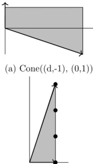
(a) Cone((d,-1), (0,1))
(b) The dual cone Cone((1,0), (1,d)) and gener- ators of the corresponding semigroup
Figure 3.1: A rational normal curveCd
Example 3.1.3. Let’s investigate the rational normal curve of degree d Cd⊆Pd using two different sets of lattice points. This example shows that two different affine cones appear, though the same projective toric variety comes from different sets of lattice points.
Let A = {(d,0),(d−1,1), . . . ,(0, d)} ⊆ Z2. Then we now can construct both the affine toric varietyYA and the projective toric varietyXA. On the other hand,Cbd=YA sinceI =I(YA), where
I =hxixj+1−xi+1xj |0≤i < j ≤d−1i,
and Cbd=V(I). The ideal I is homogeneous so that it induces a projective varietyCd, and we haveXA =Cd. Thus,A gives the result satisfying Proposition 3.1.2. Also, note that the character lattice of the torus ofYA is ZA.
However, if we take a different set B = {(0,1, . . . , d−1, d} ⊆ Z and consider the map
ΦB:C∗ −!Pd, t7!(1, t, . . . , td−1, td),
then we have XB =Cd. But, since x21−x2 vanishes at (1, t, . . . , td−1, td)∈Cd+1 for all t∈Cd+1,I(YB)⊆C[x0, . . . , xd] is not homogeneous so thatYB 6=Cbd.
Dimension of Projective Toric Varieties.Determining the dimension of projective toric varieties needs the rank of the corresponding character lattice. As the character
latticeMn ofTPn, for given A ={m1, . . . , ms} ⊆M, we set Z0A =
s
X
i=1
aimi |ai∈Z,
s
X
i=1
ai = 0
.
The rank of Z0A is the dimension of the smallest affine subspace of MR containing the set A. This lattice becomes the character lattice of the torus of a projective toric varietyXA. As in the previous example, if the affine coneXbA is not equal to the affine toric variety YA, then the rank of ZA is just the dimension of XA, whereas if the condition in Proposition 3.1.2 satisfies, homothety can be reduced from YA so that we have dimXA = rankZA −1.
3.2 Polytopes and Projective Toric Varieties
Before we begin our study, much of detailed discussion about polytopes are in [22, 23, 24].
Thedimensionof a polytopeP ⊆MRis the dimension of the smallest affine subspace ofMRcontainingP.Faces, facets, edges andvertices are defined in similar way to those of polyhedral cones.
When P isfull dimensional, each facetF has aunique supporting affine hyperplane.
We write the supporting affine hyperplane and corresponding closed half-space as HF ={m∈MR| hm, uFi=−aF} and HF+={m∈MR| hm, uFi ≥ −aF}, where (uF, aF) ∈NR×Ris unique up to multiplication by a positive real number. We calluF aninward-pointing facet normal of the facetF. Then a full dimensional polytope P has the unique presentation
P = \
F facet
HF+={m∈MR| hm, uFi ≥ −aF for all facets F ≺P}. (3.2.1) Very ample Lattice Polytopes. A lattice polytope P is the convex hull of a finite set S ⊆ M. It is equivalent to that all vertices lie in M. In this case, aF corresponding to the unique ray generator uF in (3.2.1) is integral. Before introducing the notion of very ampleness, we consider the lattice points kP ∩M for all k∈ N. If we do not lose any point when we add two sets of such lattice points with different multiplication of a polytope, then we say that such polytope hasenough lattice points.
Definition 3.2.1. A lattice polytope P ⊆MR isnormal if (kP)∩M+ (lP)∩M = ((k+l)P)∩M for all k, l∈N.
An important result on normality from [25] is given.