The copyright of this report belongs to the author under the provisions of the Copyright Act 1987 as qualified by the Intellectual Property Policy of Universiti Tunku Abdul Rahman. First, I would like to thank Universiti Tunku Abdul Rahman for the opportunity to complete this research and the necessary equipment and facilities. The study was completed with the assistance and support of friends who helped me when I encountered problems with this assignment.
It is intended to integrate a newly developed automated surface roughness data analysis program that interfaces with a surface profiler prototype.
Background
The degree of random surface roughness is determined by statistical characteristics judged by the wavelength units of the sensing sensor (Campbell and Wynne, 2011). The research was inspired by the application of understanding the surface roughness parameters by Dr. Developing a non-contact measurement is expensive; the accuracy of the sensor can be affected by many factors.
No program on the market today can automatically determine surface roughness metrics such as autocorrelation length and RMS height from raw data input.
Aims and Objectives
Measure filter reliability and accuracy by optimizing the raw data and creating a graph.
Overview
Physical Planning and Design
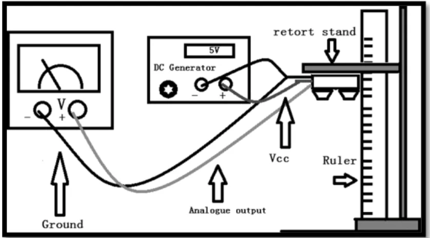
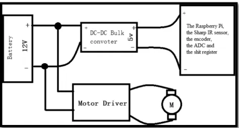
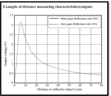
After plotting the average chart, a power function trendline is added to the chart. 11 To derive the voltage-to-distance equation, x is moved to the left side of the equation and y to the right side through a series of mathematical calculations. An ADC is required to convert the analog signal from the Sharp IR distance measurement sensor.
The input to this bulk converter module is supplied with 12 V and 5 V is obtained by adjusting the rheostat using a voltmeter attached to the output of the module.
Software Specifications
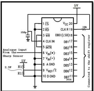
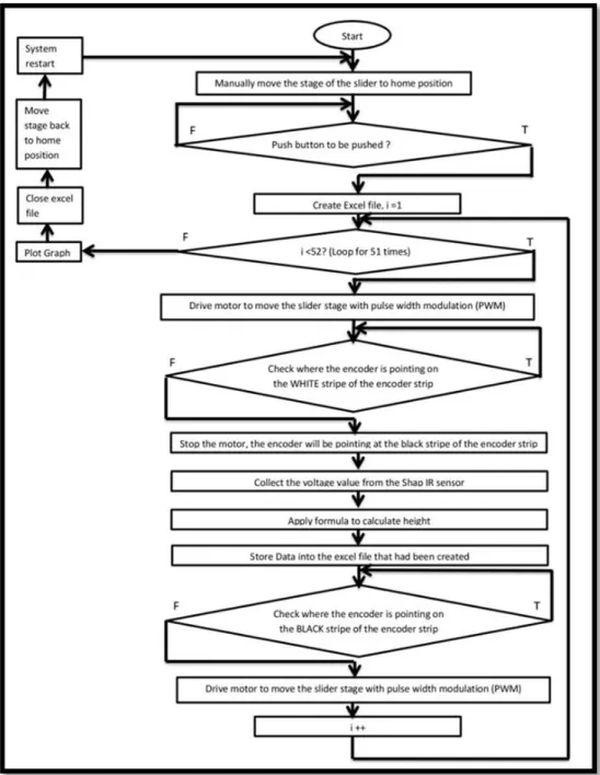
16 To calculate the height of the surface, it is necessary to retrieve data from the Sharp IR sensor using ADC and shift register. The code "import xlsxwriter" is placed at the beginning of the script to import the library. For this software to work, the IP address of the Raspberry Pi must be obtained.
Since the largest fluctuations of the graphs are less than 0.5 cm, the result obtained is considered satisfactory.
Graph Optimisation
Moving Average Filter
Thus, median filtering is an optimization process where the output of the filter is always set to the minimum of a cost function of the output state of the filter. If the output of the filter is the same as its neighbor input,𝑉𝑉𝑖𝑖(𝑛𝑛) = 𝑏𝑏𝑖𝑖(𝑛𝑛+𝑗𝑗),𝑗𝑗 ≠ 0), the median cost function is reduced. If the filter's output deviates from its neighbor, 𝑉𝑉𝑖𝑖(𝑛𝑛)≠ 𝑏𝑏𝑖𝑖(𝑛𝑛+𝑗𝑗),𝑗𝑗 ≠0), the median cost function increases.
The standard deviation of the surface height fluctuation (or RMS height) and the surface correlation length are the two most commonly used measures to assess surface roughness (Ulaby, Moore, and Fung, 1981).

Surface Autocorrelation Length
Programming Languages
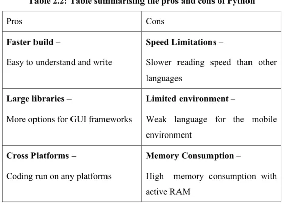
In the extreme case of a perfectly smooth surface, every point on the surface is correlated with every other point by a correlation coefficient of unity. Python's efficiency in multiple technical domains argues for the reason for such a large and active Python community (upGrad, 2021). Python has a library that allows the developer to detect and display the mouse and keyboard inputs (Shepherd, 2020).
Because of its security, maintainability, platform independence and many other benefits, Java is one of the most widely used languages in the software industry (BairesDev, 2022). C++ is widely used as it can be run as a C program without changing the code.
GUI Frameworks
Tkinter
It is the most widely used Python GUI framework as it is a mature framework that offers many widgets such as canvas, graph generation and popup messages.
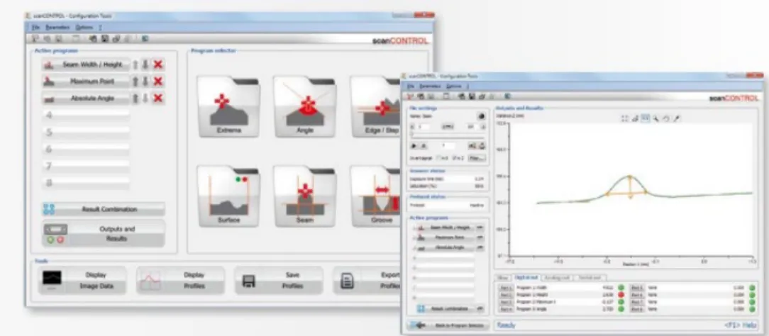
Existing Surface Profiler Analysis Software
Google Drive
Drive connects to Docs, Sheets, and Slides, cloud-native collaboration apps that help the team produce content more effectively and collaborate in real time. Collaborate in Microsoft Office files without converting file formats, and edit and store over 100 different file types, including PDFs, CAD files, and images (Google, 2019).
Comparison of features
Overview
Selection of Programming language
44 Since its debut in 1995, Java has been the most popular and sought-after programming language. Python has reached the top three most popular programming languages within a few years as its popularity increases annually. Python has a built-in standard library known as TK (Tkinter for GUI interface), another feature.
GUI Framework Selection
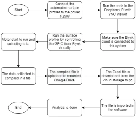
The system flow diagram between hardware and software is shown in Figure 3.1 below. The ProSight Surface Profiler software is an automated system that reads data from a surface profiler data file. Users can easily move the graph to increase the efficiency and effectiveness of the analysis task.
In addition, users can save the chart as an image for archival purposes and distribute it to whomever they want. The .exe extension of the software allows the developer to send the download link directly to the engineer.
Real-time analysis
Data View
Graph generated
Saved data
Hardware
Software
Graph Optimisation
- Moving Average Filter
- Savitzky-Golay Filter
SciPy does not have a built-in implementation of a moving average filter, but it is easy to implement. A moving average of order 𝑛𝑛 has an impulse response with 𝑛𝑛 elements that all have the value 1/𝑛𝑛. It is a scalar or list of length N that gives the average filter window size in each dimension.
If 𝑘𝑘𝑚𝑚𝑒𝑒𝑛𝑛𝑚𝑚𝑙𝑙_𝑒𝑒𝑖𝑖𝑧𝑧𝑚𝑚 is a scalar, then this scalar is used as the magnitude in each dimension (Virtanen et al., 2020). As the value of 𝑛𝑛 increases, the optimized graph eliminates the spikes and calculates the average height of the newly generated spikes to obtain the actual height of the element. The Savitzky-Golay filter calculates a polynomial fit of each window based on the polynomial degree and window size.
As the value of polynomial order increases, the optimized graph does not eliminate the spikes. As you move upwards, the gradient of the optimized graph is sloping, which is a negative result. All the optimized graph of polynomial order = 5, 7 and 9 show the sloping line when going up to 4−6 𝑐𝑐𝑚𝑚.
After comparing the three filters, the most accurate and suitable is the median filter with an n value of 9. For the moving average filter and the Savitzky-Golay filter, both filters gave a negative result because they do not remove spikes uniformly and the height surface is not flat like the actual object.
RMS Height
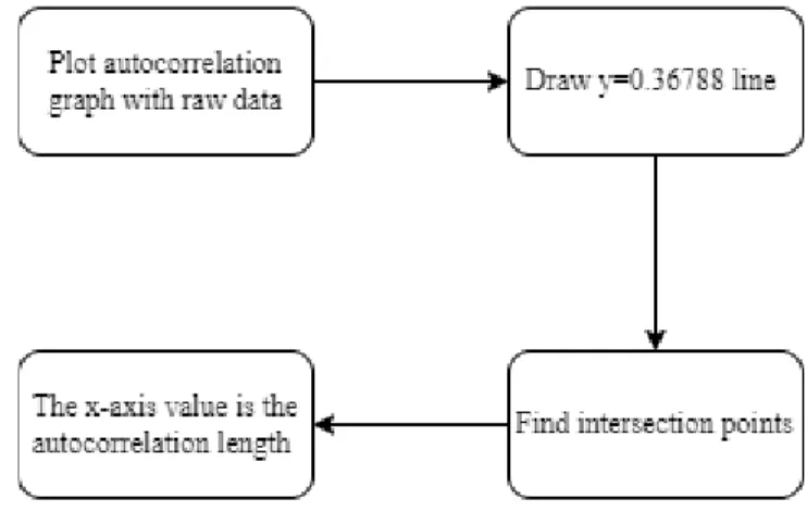
The plot shown in Figure 3.9 below is a plot of the autocorrelation function (blue line) with the raw data from the snow site. The orange dot is the intersection between the horizontal line y=0.36788 and the graph of the autocorrelation function. The plot of the autocorrelation function is plotted using the tsaplots.plot_acf( ) function from the Statsmodels library.
The x-axis shows the number of delays and the y-axis shows the autocorrelation at that number of delays. The intersection is found using a library called "shapely.geometry" which imports a function called LineString. The function separated the graph of the autocorrelation function and the horizontal line of y=0.36788 into 2 lines, then locates the intersection of both.
Selection of the IoT platform
- Import of library
- Debugging errors
- Global definition
- Widgets for Homepage (Class II)
- PageOne (Class III)
- Design of PageTwo (Class IV)
- Setup for an executable extension
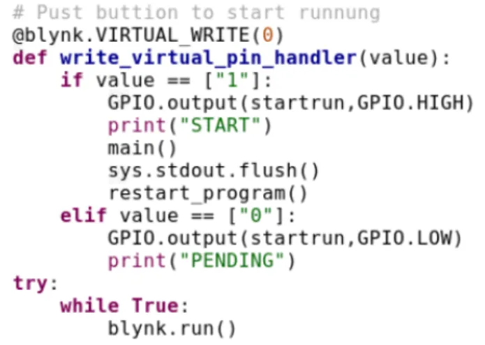
As shown in Figure 3-13, a function has been written to manage the Raspberry Pi's GPIO pin. Therefore, a command line is coded, as shown in Figure 3-22, to change the recursion limit in Python. The image below, shown in Figure 3.24, is the global definition code to be used in the program.
Two lines of code are called to run the entire system, as shown in Figure 3-46 below. The code shown in Figure 3.47 below is executed to generate an executable extension (.exe) for installation.
Introduction
Surface Roughness Parameter
- Surface Roughness Parameters (Software Algorithm)
The calculated parameters and the autocorrelation function graph for 8 sites are shown in Tables 4.1 and 4.2 below. The parameters and autocorrelation function graph for 8 locations from the software algorithm are shown in Tables 4.3 and 4.4 below. Based on the results obtained from the software algorithm for autocorrelation length and RMS height, the percentage error is calculated as shown in Tables 4.5 and 4.6.

Graph optimisation
- Case Study 2
- Case Study 3
- Case Study 4
- Case Study 5
- Case Study 6
- Case Study 7
- Case Study 8
- Summary of the case study of graph optimisation
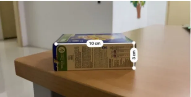
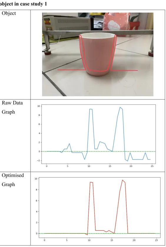
The object shown in Table 4.7 below is drawn with the red line to visualize the expected outcome of the graph. The object shown in Table 4.8 below is drawn with a red line to visualize the expected outcome of the graph. The object shown in Table 4.9 below is drawn with a red line to visualize the expected outcome of the graph.
92 Table 4.9: Plot of raw data compared to optimized plot with the following object in case study 3. The object shown in Table 4.10 below is drawn with a red line to visualize the expected result of the plot. The object, as shown in Table 4.11 below, is drawn with a red line to visualize the expected output of the graph.
Table 4.11: Raw data graph compared to the optimized graph for the next object in Case Study 5. The object in Table 4.12 below is drawn with a red line to visualize the expected outcome of the graph. The object in Table 4.13 below is drawn with a red line to visualize the expected outcome of the graph.
98 Table 4.13: Plot of raw data compared to optimized plot with the following object in case study 7. The object shown in Table 4.14 below is drawn with a red line to visualize the expected result of the plot.
Conclusion
The measured data output is inconsistent and the data cannot be precisely optimized. Further, the contactless system cannot be implemented without a WIFI connection because the Blynk app and Google Drive require an internet connection.
Recommendations for Future Improvement
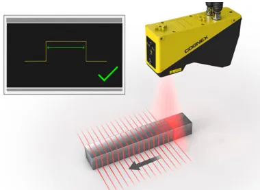
Available at: https://www.cognex.com/products/machine-vision/3d-machine-vision- systems/in-sight-laser-profiler/software [Accessed: 15 April 2022]. Available at: https://www.theserverside.com/tip/Five-tips-for-choosing-a-UI- development-framework [Accessed: 15 April 2022]. Available at: https://www.micro-epsilon.com/2D_3D/laser-scanner/Software/scanCONTROL-Configuration-Tools/ [Accessed: 15 April 2022].
Available at: https://www.upgrad.com/blog/reasons-why-python-popular-with-developers/#Why_is_Python_becoming_so_popular_in_this_decade [Accessed: April 15, 2022].