Samsul Ariffin Abdul Karim Jabatan Sains Asas dan Gunaan, Pusat Penyelidikan Tenaga Grid Pintar (CSMER), Institut Sistem Autonomi, Universiti Teknologi PETRONAS, Seri Iskandar, Perak Darul Ridzuan, Malaysia. Mahmod Othman Jabatan Asas dan Sains Gunaan, Universiti Teknologi PETRONAS, Seri Iskandar, Perak Darul Ridzuan, Malaysia.
1 Introduction
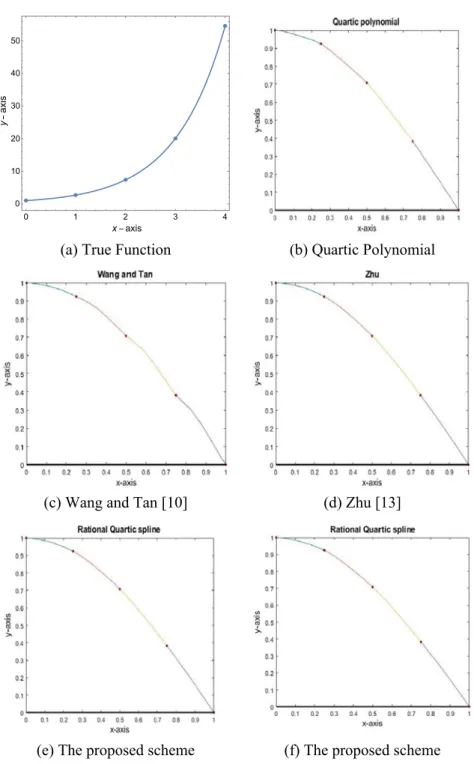
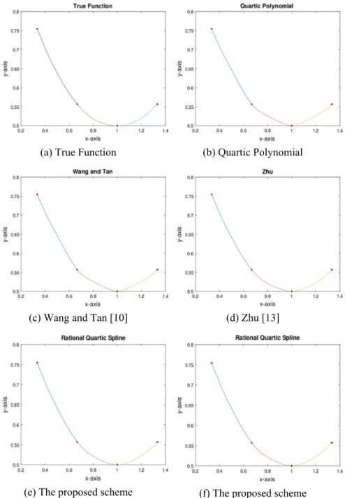
Furthermore, an application in signal processing shows that the proposed RQS is very accurate for upsampling the discrete-time signal. The error evaluation shows that the proposed scheme gives higher accuracy in terms of the smallest error compared to the quartic polynomial scheme, Wang and Tan [6] and Zhu [11].
2 Construction of Rational Quartic Spline Interpolant
- Rational Quartic Spline (RQS)
- Derivative Estimation
- Derivative Estimation
- Convergence Analysis of RQS
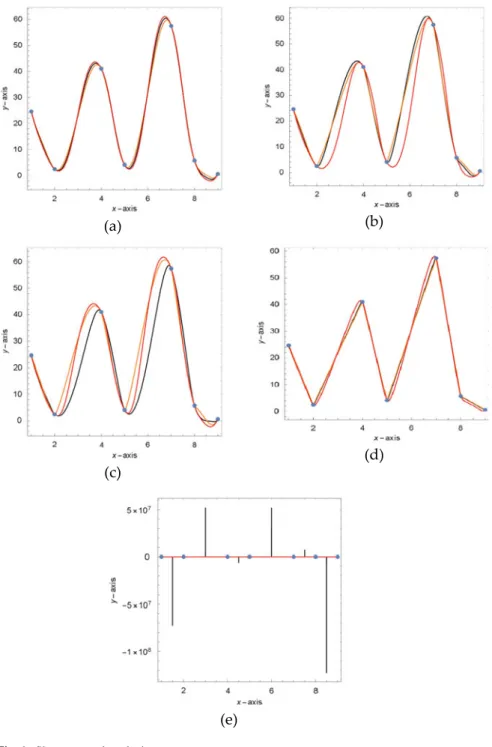
At the endpoints ofx1andxn. n−1 value of day is given as. 1), some observations can be made as follows: a) The RQS scheme in Eq. d) The RQS scheme in Eq. Figure 1 represents the interpolation curve obtained by the proposed scheme using the parametric values given in Table 2 .
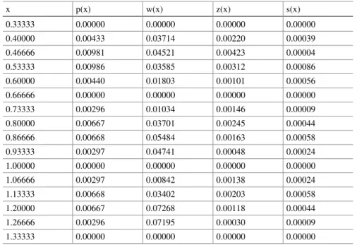
![Table 1 Data from [14]](https://thumb-ap.123doks.com/thumbv2/azpdforg/10414361.0/18.659.80.581.97.167/table-1-data-from-14.webp)
3 Data Interpolation Using RQS
Simulations have been performed several times, and the parameters shown in the tables listed below are the best numerically. MATLAB version 2019 installed on Intel® Core™ i5-8250U @ 1.8 GHz CPU is used to produce all graphical and numerical results.
![Table 3 Data from [15]](https://thumb-ap.123doks.com/thumbv2/azpdforg/10414361.0/22.659.86.576.803.888/table-3-data-from-15.webp)
4 Discussion
It can be observed that Wang and Tan [10] have the highest maximum absolute relative error followed by quartic polynomial, Zhu [7] and the proposed scheme. For the proposed schemes, 1(x) has the smallest absolute error compared to some other existing schemes.
5 Applications in Signal Processing
Based on the numerical error analysis, we conclude that the proposed RQS is better than the existing rational quartic splines interpolation with the smallest error. Based on this figure, the proposed RQS still gives a very good result even though we only use 8 samples.
6 Conclusion
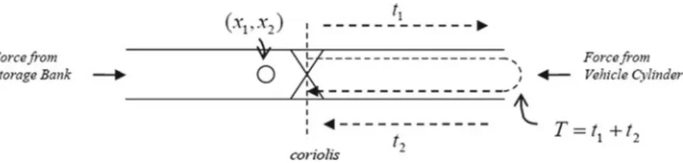
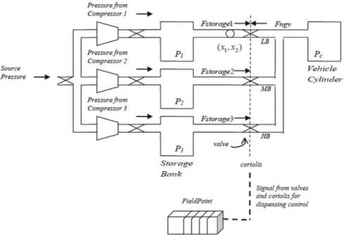
Dispenser with Multi-Level-Pressure Banks
The results revealed the robustness of the proposed TOC refueling algorithm when used in NGV refueling using multi-level pressure banks. One of the pioneering works dealing with the optimal time switching problem dates back to Kuo et al.
2 NGV Dispenser Model
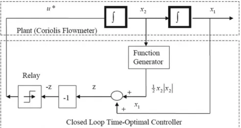
3 Time-Optimal Control Model of NGV Dispenser
- Parameter Identification
- Development of Switching Time Equation
- Designing Governing Equations
- Implementation of Pontryagin’s Minimum Principle
- Designing Forced Trajectory
- Derivation of Optimal Switching and Total Minimum Time
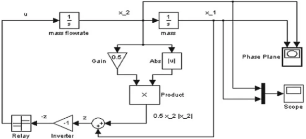
- Modeling of Forced Trajectory Using MATLAB/Simulink
- Simulation Example
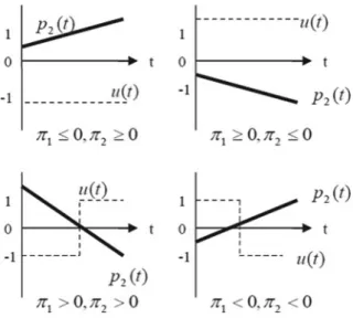
For the control problem, the objective is to take each initial state to (0,0), that is, the origin of the state plane. Let R+ be the region of points to the left of the commutator curve γ such that R+=.
4 Results and Discussion
Performance of Refueling by Varying Initial Pressure Inside Receiver Tank
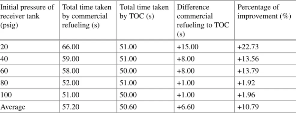
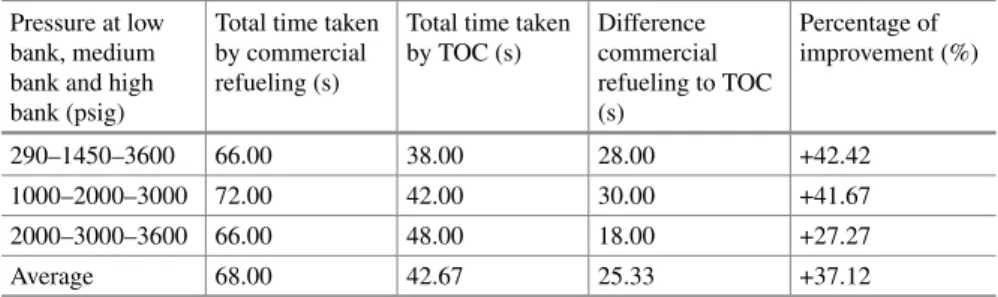
As shown in Tables 2 and 3, the TOC fueling time for a range of initial pressures from 20 to 100 psig would be faster than commercial fueling by an average difference of 6.60 s and an average total mass loss of 0.04 kg. The results confirm that at lower initial pressure ranges, i.e. 20-100 psig, TOC fueling is superior in terms of fueling time, while at higher initial pressure ranges Table 2 Analysis of total time comparison between commercial fueling and TOC fueling at initial receiving tank pressures ranging from 20 to 100 psig.
Performance of Refueling Using Multi-Level-Pressure Storage Banks
Interestingly, the results show that the TOC refueling time is much faster than commercial refueling, with an average difference of 25.33 s and a total mass loss of only 0.95 kg. The results verify the viability of TOC compared to commercial fueling when used as a switch controller in fueling NGVs using multi-level pressure storage banks.
5 Conclusion
Park, M.G., Cho, N.Z.: Time-optimal power control of nuclear reactors with adaptive proportional-integral feed forward gains.
Tracking System in UTP
This leads me to my research to analyze the performance and effectiveness of single-axis and fixed-axis solar tracking system. To develop a prototype single-axis solar tracking system using an active closed-loop system.
2 Related Literature Review
The results show that the solar tracking system can produce 40% more energy than a fixed-axis solar tracker. This shows that daily adaptation can produce more energy and power compared to a conventional tracking system.
3 Project Flow and Methodology
4] An experiment on the concept of a solar tracking system was conducted to determine how the sun's position is tracked by the sun's orientation and inclination. It can also be used as a guide to the operation of the solar tracking system and the limitations of the system.
4 Data Collection
At night, the LDR will detect low light intensity and turn off the system (Fig.3). The adjustment of the LDR sensor plays a crucial role, if the adjustment of the LDR sensors is not done correctly, it will cause trouble for the LDR to detect the position with the highest light intensity and send the information to the Arduino so that the solar panel can move in that particular place.
5 Results and Discussions
In the single axis solar tracking system, there is only one linear actuator that controls the movement of the solar photovoltaic panel from east to west. At noon, the current and voltage produced by the single-axis solar tracker and the fixed solar panel are the same. This is because the position of the solar panel is perpendicular to the sunlight.
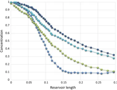
The model gives a better understanding of the geochemical phenomenon and the spatial distribution of the movement of fine particles and nanoparticles in porous media [21-25]. The present study focused on developing a simplified model for nanoparticle flow in porous media and the effect of fine migration on nanoparticle adsorption in porous media.
2 Mathematical Modeling of Nanoparticles Flow in the Reservoir
The material balance equation for the flux concentration of nanoparticles in a porous medium is given by [23,24]. Fluid flow in a porous medium describes the energy contained in the flow of nanoparticles; it is shown as Equation 3.
3 Data Collection
First, Eq.1 is solved with the above initial and boundary conditions, and then the fine particle concentration is solved using Eq.2, which leads to the solution of Eq.1. Using the solution of Eq.1, the concentration of nanoparticles is calculated using Eq.2 with the same initial and boundary conditions.
4 ANN Model Development
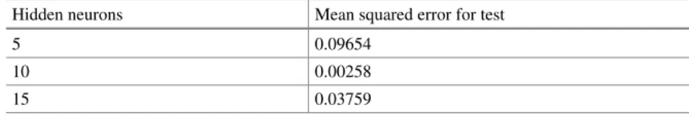
The variable, also called the objective variable, is the comparative estimate of the concentration of the nanoparticles. In this study, the mean square error (MSE) and correlation coefficient (R) were used to evaluate the model performance.
5 Results and Discussion
The parameters of the given neural network model are characterized by weights (w) and biases (b) that connect the different layers. The learning, then testing and finally generalization are the three fundamental steps to obtain the optimal ANN model.
Appendix: ANN Matlab Code
Habibi, A., Ahmadi, M., Pourafshary, P., Ayatollahi, S., Al-Wahaibi, Y.: Reduction of fine particle migration by nanofluid injection: an experimental study. Yuan, B., Moghanloo, R.G., Zheng, D.: Analytical evaluation of the use of nanoparticles to mitigate the migration of fine particles in porous media.
System Towards Sustainability: Taylor’s University as the Case
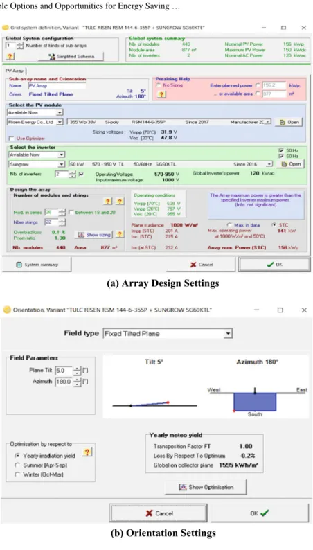
The load curve of the transformers in TULC is based on energy audit data and is maximum active. Based on TULC's monthly electricity bill, the average maximum demand is 3061 kW over the 12 months in the year 2017.
2 PV Installation Option
The highest share of the total energy consumption is usually from the chiller, the commercial block and the hospital building. This software is commonly used in the industrial sectors to predict PV system performance with loss assumption calculation.
3 Orientations of the Placements of the PV
Dimensioning of PV array is done by defining the selection of the PV modules in the library and the specification of losses. It has a big impact on the system performance because it has inverter efficiency loss which is considered as one of the major efficiency losses in the system.
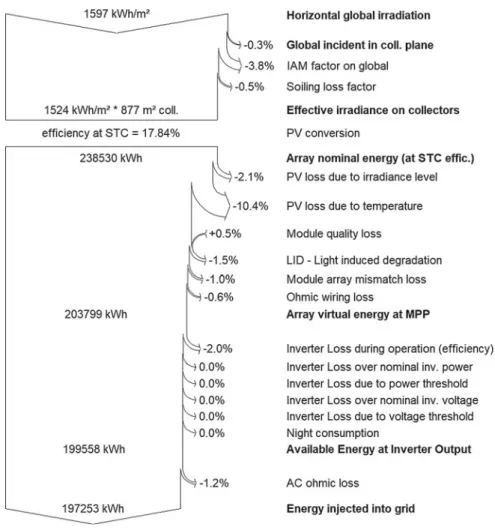
4 Energy Flow Analysis
As a result of using the PV system software, the performance ratio is 79.3%, which means that 20.7% of the energy generated through the PV panels is lost in the system losses.
5 Economic Analysis
With the annual specific yield obtained from the results of the PV systems based on the size of the system, the annual solar generation from the system is 197,028 kWh. The PV array is sized using the PV systems software with the loss diagram shown.
C Surface Interpolation Using Quartic Rational Triangular Patches
The main purpose of sparse data interpolation is to produce a surface which achieves some degree of smoothness between two adjacent triangles. All the existing schemes used in sparse data interpolation do not have any free parameters for shape preservation.
2 Rational Quartic Triangular Patches
In addition, we investigate the influence of the shape parameters on the smallest RMSE, maximum error, and CPU time (in seconds).
3 C 1 Continuity Between Two Patches
4 Error Calculation
5 Numerical Results and Discussion
Spline Tensor Product Scheme
- Literature Review
27] present a family of (2n−1)-free-parameter binary point approximation subdivision schemes for describing curves. In 2014, Mustafa and Bari [29] worked on the new family of non-stationary singular point subdivision schemes, using Lagrangian identities.
2 Preliminaries
Properties of the Scheme
- Smoothness of the Scheme
- Holder Exponent
- Polynomial Generation and Reproduction
To prove the continuity of the subdivision scheme Sξ related toξ(x), we need to prove the convergence of d1(x). In this section we will talk about the degree of polynomial generation and polynomial reproduction of the Septic B-spline scheme.
3 Construction and Analysis of Septic B-Spline Tensor Product Scheme
Preliminaries
In the case of bivariate subdivision scheme, there are four rules depending on the parity of each component in the multi-index u=(u1,u2). Since there are four rules for calculating the values at the next refinement level, we define the norm as:
Construction of Septic B-Spline Tensor Product Scheme
Ifb(x1,x2)=b(x2,x1), which is typical of schemes with the symmetry of the square lattice, then ξ(x1,x2)=ξ(x2,x1), and the contractivity of only one form be checked.
Analysis of Septic B-Spline Tensor Product Scheme
4 Numerical Examples
Here, we have provided the B-spline septic subdivision approximation scheme using the symbolic form of the Laurent polynomial method to determine the smoothness of our scheme. Kanwal, G., Ghaffar, A., Hafeezullah, M.M., Manan, S.A., Rizwan, M., Rahman, G.: Numerical solution of 2-point boundary value problem by subdivision scheme.
Uncertainty Within Gaussian Framework for Seismic Inversion
We estimate the norm of the difference between the exact solution me and the regularized onemaδ =Rαdδby. By virtue of the property of the regularizing family (1), the first term on the right-hand side of (4) tends to zero whenα→0, i.e.
3 Bayesian-Tikhonov Formulation for Linear Inverse Problems
From Bayes' theorem, we can determine our posterior density from the product of the likelihood and the a priori densities. From the point of view of the Tikhonov regularization, the first term checks the closeness of the solution to the observed data and the second one acts as a penalty.
4 The Maximum a Posteriori (MAP) Point
In order to provide a balance between these two terms, the choice of theλ is a non-trivial challenge in Tikhonov regularization. In general, Tikhonov regularization solution is the outcome of a balance between fitting the data and eliminating unwanted features.
5 A Generalised Formulation
We will introduce the concept of filter factors as a measure of the balance between information from observed data versus a priori information in determining parameter estimates. The corresponding SVD components specify well-resolved directions or directions of certainty about the observed data compared to the a priori information.
6 The a Posteriori Covariance Matrix
The observed data fully determines the solutions, that is, the likelihood function fully determines the shape of the a posteriori PDF. The singular valuesσi2 resulting from the forward modeling are inversely proportional to the noise levelγ2 in the observed data.
7 The Resolution Matrix
Based on the two extreme situations described above, the a posteriori covariance matrix must take into account the interactions between the information from the observed data and the a priori information. Based on these extreme situations, the resolution matrix is a measure of the balance between the information from the observed data compared to the a priori information in determining the parameter estimates, as we defined earlier.
8 The Optimal Low-Rank Approximation of a Posteriori Covariance Matrix
Hence, it provides the balance criterion we need to approximate the optimal a posteriori. determination of the boundary between information provided by measurements in the observed data with respect to the previous information. To facilitate the determination of the boundary between information provided by measurements in the observed data with respect to the preceding information of the singular value spectrum, we can relate this to the concept of filter factor introduced in Sect.4.
9 Numerical Examples
The first column in Figure 4 represents the prior variance and its approximation of the mean model without information from the observed data. 4 First column: The prior variance field and its approximation of the mean model without information from the observed data.
10 Conclusions
Flath, H., Wilcox, L., Akçelik, V., Hill, J., van Bloemen Waanders, B., Ghattas, O.: Fast algorithms for Bayesian uncertainty quantification in large-scale linear inverse problems based on low-rank partial hessian approaches. Spantini, A., Solonen, A., Cui, T., Martin, J., Tenorio, L., Marzouk, Y.: Optimal low-level approximations to Bayesian linear inverse problems.