CHAPTER 1 INTRODUCTION
1.1 Background
It is certainly true that the presence of interfacial shearing tractions has only a very small effect on contact pressure distribution. But, in the real case, the tractions give significant impact to the surface between these contacts. In order to prove the influence of tractions to sliding complete contact, an analysis is going to be carried out using computerized software of finite element analysis.
1.2 Problem Statement
During sliding between two bodies of elastically similar complete contacts, the stresses at the edge of complete contacts are severe. The regions where the stresses are severe are of high possible sites of crack nucleation which can lead to defect of components.
1.3 Objective
The objectives of this project amongst others are modelling of sliding contact problem and determination of contact parameters at the contacting surface and also at the edge of the contacts. Subsurface stresses of the contact also need to be analyzed.
1.4 Scope of Study
This analysis is about studying method of solving contact problem between two similar elastic bodies. This problem is modelled and analyzed using Finite Element Analysis (FEA). It involves usage of computer software ANSYS. This software is used to simulate the sliding contacts and from the simulation itself, region of critical stresses will be obtained and analyzed.
CHAPTER 2
LITERATURE REVIEW/THEORY
2.1 Introduction
2.1.1 Theory of Contact – Contact Mechanics
Contact mechanics is an area of physics in which the motion of two or more bodies in space is restricted by additional constraints. These so called unilateral constraints ensure that bodies once coming into contact do not penetrate each other. Once the general equations for a contact problem are set up, different solution schemes can be used to simulate the behavior of bodies in contact and to compute displacement and stress fields. There are several possibilities to classify contact problems. Generally contact with and without friction is distinguished.
In case of analytical solution methods for contact problems the following classification was introduced. Contact may occur between bodies in two distinct ways. A conforming contact is one in which the two bodies touch at multiple points before any deformation takes place or in other words, they just "fit together”. The opposite is non- conforming contact, in which the shapes of the bodies are dissimilar enough that, under no load, they only touch at a point or possibly along a line. In the non-conforming case, the contact area is small compared to the sizes of the objects and the stresses are highly concentrated in this area.
Such distinctions however do not have to be made when numerical solution schemes are employed to solve contact problems. These methods do not rely on further assumptions within the solution process since they base solely on the general formulation of the underlying equations. Besides the standard equations describing the deformation and motion of bodies to additional inequalities can be formulated. The first simply restricts the motion and deformation of the bodies by the assumption that no penetration can occur. Hence the gap gN between two bodies can only be positive or zero
where gN = 0 denotes contact. The second assumption in contact mechanics is related to the fact, that no tension force is allowed to occur within the contact area (contacting bodies can be lifted up without adhesion forces). This leads to an inequality which the stresses have to obey at the contact interface. It is formulated for the contact pressure
Since for contact, gN = 0, the contact pressure is always negative, pN < 0, and further for non contact the gap is open, gN > 0, and the contact pressure is zero, pN = 0, the so called Kuhn-Tucker form of the contact constraints can be written as
These conditions are valid in a general way. The mathematical formulation of the gap depends upon the kinematics of the underlying theory of the solid (e.g., linear or nonlinear solid in two- or three dimensions, beam or shell model),
Complex forces and moments are transmitted between the bodies where they touch, so problems in contact mechanics can become quite sophisticated. Typically, a frame of reference is defined in which the objects (possibly in motion relative to one another) are static.
They interact through surface tractions (or pressures/stresses) at their interface. As an example, consider two objects which meet at some surface S in the (x,y)-plane. One of the bodies will experience a (normally-directed) pressure p = p(x,y) and (in-plane) surface traction q = q(x,y) over the region S. In terms of a Newtonian force balance, the forces:
and
must be equal and opposite to the forces established in the other body. The moments corresponding to these forces:
are also required to cancel between bodies so that they are kinematically immobile.
2.1.2 Modelling of Sliding Contacts
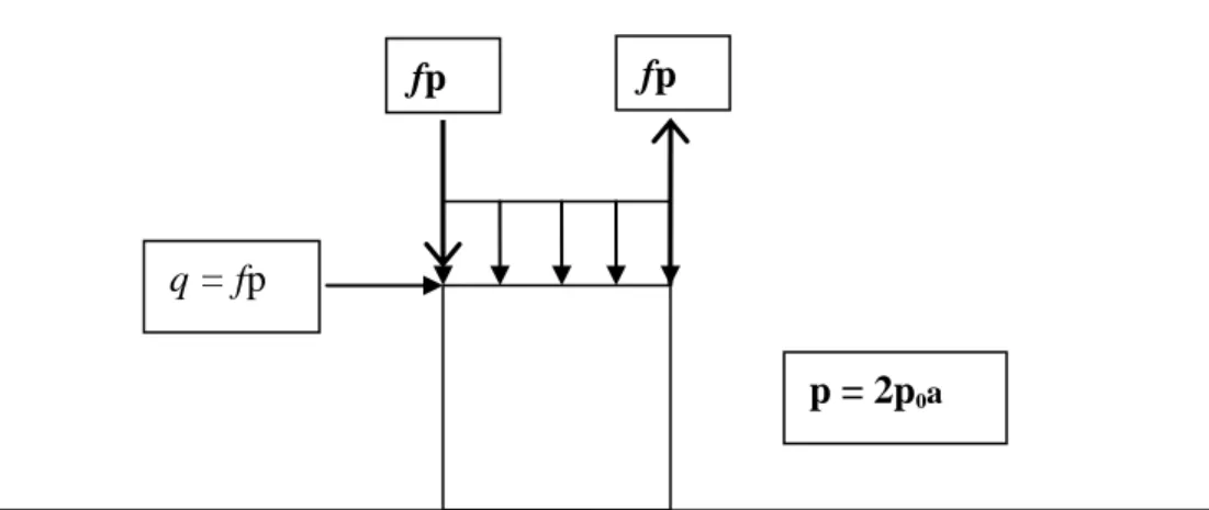
In this analysis, the sliding contact problem is modelled by using a square punch and a half plane. Geometry of the contact problem is shown in Figure 2.1 below. Note that the square punch has a dimension of of 2a x 2a. Pressure, p is applied on the upper side of the punch onto an elastically similar half-plane. In order to make the punch slides, shearing force, q is applied just enough to cause sliding [1].
Figure 2.1: Geometry of the contact
2.1.3 Failure at the Contact Interface
Contact problem are commonly found in engineering problems. These problems include splint joint between shafts, bolted connections. Specifically, in condition where sliding contact may occur, type of failure that will occur is fretting fatigue failure [2].
How this failure affected the components in contact is, they reduce the fatigue life and endurance limit of the mechanical components. One example was taken from an experiment of fretting fatigue failure involving titanium alloy.
fp fp
q = fp
p = 2p0a
2.2 Sliding Contact and its modelling in Analysis
Sliding contact is commonly found in many engineering problems. Examples of situation where sliding contact can occur are in shaft splint joints and bolted connections.
In this analysis, the sliding contact is modelled by a sliding square-ended punch in contact with an elastically similar half plane. Both of that square punch and half plane are shown in the figure 2.1. There are some forces and moments need to be applied on the model so that it can make a contact and slides. Firstly, pressure need to be applied along the top line of the punch in order for it to touch with the surface of the half plane and make contact with it. Then a shearing force, q will be applied on the top line too just to make the punch slide along the half plane. In addition with this shearing force is the anti- clockwise moment which is also applied on the same line with the shearing force (Refer to Figure 2.1). This is to prevent the square punch from overturning [1].
During sliding of elastically similar complete contacts, there are tractions at the contacting surface. This can be modelled by a square block sliding along an elastically similar half plane, in the presence of friction.
2.3 Finite Element Analysis (FEA)
FEA uses a complex system of points called nodes which make a grid called a mesh. This mesh is programmed to contain the material and structural properties which define how the structure will react to certain loading conditions. Nodes are assigned at a certain density throughout the material depending on the anticipated stress levels of a particular area. Regions which will receive large amounts of stress usually have a higher node density than those which experience little or no stress. Points of interest may consist of: fracture point of previously tested material, fillets, corners, complex detail, and high stress areas. The mesh are interconnection between nodes and act like a spider web in that from each node, there extends a mesh element to each of the adjacent nodes. This web of vectors is what carries the material properties to the object, creating many elements.
2.3.1 Nonlinearity in contact analysis
Contact between two bodies exhibits nonlinear solutions. Nonlinear solutions means, in a structure being analyzed using finite element analysis, the loading causes significant changes in stiffness and the strains are beyond the elastic limit. There are two types of nonlinearities which are geometric and material nonlinearities. Geometric nonlinearities involve nonlinearities in kinematic quantities such as the strain- displacement relations in solids. Such nonlinearities can occur due to large displacements, large strains, large rotations, and so on. The contact problem under consideration can also be classified as a geometric nonlinearity because the area of contact is a function of the deformation.
2.4 Stress Analysis Using FEA Software – ANSYS
ANSYS will be used in this project. ANSYS is a comprehensive general-purpose finite element computer program that contains over 100,000 lines of code. ANSYS is capable of performing static, dynamic, heat transfer, fluid flow and electromagnetism analysis.
There are three processors that are used most frequently:
I. Preprocessor
The preprocessor contains the commands needed to create a finite element model. The process flows in this stage are as follows:
a. Define element types and options b. Define element real constants c. Define material properties
At this point, physical properties of the material will be defined such as modulus of elasticity, Poisson’s ratio, thermal conductivity and others.
d. Create model geometry e. Define meshing objects f. Mesh the object created
II. Processor
The next step involves applying appropriate boundary conditions and the proper loading. The solution processor has the commands that allow applying boundary conditions and loads. It includes:
a. for structural problems: displacements, forces, pressures and temperature for thermal expansion.
b. for thermal problems: temperatures, heat transfer rates, convection surfaces and internal heat generation.
III. Postprocessor
Postprocessors are available for review of the results.
CHAPTER 3 METHODOLOGY
3.1 METHOD OF ANALYSIS Methodologies for this project include:
1. Understanding the objective of this project by reading journal related to sliding of complete contacts.
2. There are two methods used; analytical which is Asymptotic Method and the other is Finite Element Method by using computer software, ANSYS. Finite Element Method will be adopted in this project
3. Study on how to use ANSYS
4. Modelling of the sliding complete contacts using ANSYS 5. Simulate the model generated
6. Analyze the data from simulation and come out with conclusion and recommendation if possible
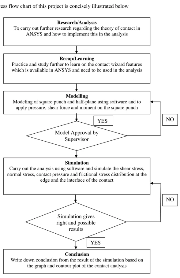
3.2 Procedure Flow Chart
Process flow chart of this project is concisely illustrated below
Figure 3.1: Flow Chart of the Project Research/Analysis
To carry out further research regarding the theory of contact in ANSYS and how to implement this in the analysis
Recap/Learning
Practice and study further to learn on the contact wizard features which is available in ANSYS and need to be used in the analysis
Modelling
Modeling of square punch and half-plane using software and to apply pressure, shear force and moment on the square punch
Model Approval by Supervisor
Simulation
Carry out the analysis using software and simulate the shear stress, normal stress, contact pressure and frictional stress distribution at the
edge and the interface of the contact
Simulation gives right and possible
results
Conclusion
Write down conclusion from the result of the simulation based on the graph and contour plot of the contact analysis
NO YES NO
YES
3.3 Contact Analysis
Initial analysis involves modeling and meshing of sliding complete contacts using ANSYS. The process requires creation of all the necessary environments, which are basically the preprocessing portions for each environment, and write them to memory.
Then in the solution phase they can be combined to solve the coupled analysis.
In general, steps involved in contact analysis using ANSYS are:
1. Create the model geometry and mesh 2. Identify the contact pairs
3. Designate contact and target surface 4. Define the target surface
5. Define the contact surface
6. Set the element KEYOPTS and real constants 7. Apply necessary boundary conditions
8. Define solution options and load steps 9. Solve the contact problem
10. Review the result
Analysis of contact between the square punch and the elastically identical half plane is done using ANSYS, utilizing the contact element analysis to simulate how the reaction between the square punch and the half plane, specifically at the interface between those two bodies. There are three main steps in order to carry out the analyses which are:
I. Preprocessing: Defining the problem
II. Solution Phase: Assigning Loads and Solving III. Post processing: Viewing the result
In every main step, there are some sub-steps involved. The whole methodology in executing the contact analysis is described below:
I. Preprocessing: Defining the problem Modeling – Define areas
Preprocessor > Modeling > Create > Area > By Dimension Table 3.3: Dimension of Contact Model
Element Dimension
Half Plane (X1= 0, X2= 20) (Y1= 0, Y2= 10)
Square Punch (X1= 9, X2= 11) (Y1= 10, Y2= 12)
Define Material Element Property
Preprocessor > Material Props > Material Models > Structural > Linear > Elastic >
Isotropic
Table 3.4: Material Properties of Contact Model
Young’s Modulus, EX: 115 GPa
Poisson’s Ratio: 0.33
Define Element Types
Preprocessor > Element Type > Add/Edit/Delete
For this analysis, we will use Structural Mass Solid, PLANE42 (Quad 4node 42) element. It is because this analysis is in 2D and the element has 2 degrees of freedom (DOF) at each node which means translation along the X and Y.
Define Mesh Size
Preprocessor > Meshing > Size Controls > Manual Size > Areas > All Areas For this analysis, an element having edge length of 1 unit is used but to get more accurate results, the element edge length is reduced to 0.1 units. Besides using manual size controls, automatic or smart size control also can be used.
Generate Mesh Frame
Preprocessor > Meshing > Mesh > Areas > Free > Pick All
Create Contact Pair Using Contact Wizard
This is the important steps of analysis because, if the contact element is successfully generated, then only ANSYS can give result of the contact analysis during the post-processing. This step is considered critical in this analysis. Contact Wizard Window will appear and steps to follow in generating the contact element is:
Main Menu> Preprocessor > Modeling > Create Contact Pair
Define Boundary Constraint
Solution > Define Loads > Apply > Structural > Displacement > On Lines
Fix the bottom end of the half plane. All degrees of freedom are constrained, meaning that the translations in X and Y axes are having zero displacement.
Apply Loads / Pressure / Moment
Solution > Define Loads > Apply > Structural > Pressure > On Lines
Apply a pressure of 100 in Y-direction to the lines at the upper side of the square punch
Solution > Define Loads > Apply > Structural > force/moment > On Lines
Apply a shear force, q, whereby q = coefficient of friction, f x pressure, p in X- direction to the lines at the upper left side of the square punch. Note that moments in both clockwise and counter-clockwise also applied to prevent the square punch from tilt from the half-plane.
Set Solution Control
Solution > Analysis Type > Sol’n Control
Solve the System
Solution > Solve > Current LS
CHAPTER 4
RESULTS AND DISCUSSION
4.1 Result
4.1.1 Surface Stress Analysis
Based on the methodology used earlier, results from the analysis are shown below.
The important parameters which need to be analyzed are:
SY – Stress in Y-direction
SXY – Shear Stress in XY-direction
Contact Pressure (contpress) along the contact interface Frictional Stress (fricstress) along the contact interface
The characteristics and results of the analysis is shown on the following pages:
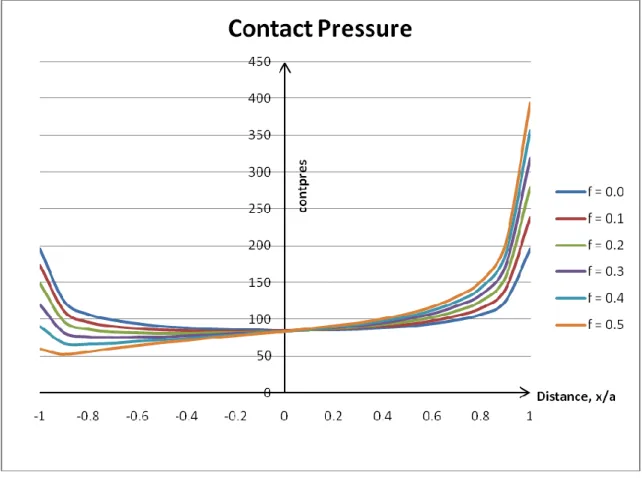
Figure 4.2: Distribution of contact pressure along the contact interface (f=0.0 until f=0.5)
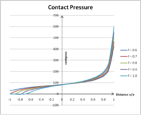
Figure 4.3: Distribution of contact pressure along the contact interface (f=0.6 until f=1.0)
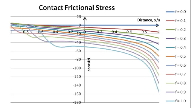
Figure 4.4: Distribution of contact frictional stress along the contact interface (f=0.0 until f=1.0)
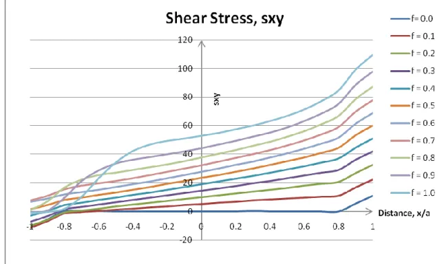
Figure 4.5: Distribution of contact shear stress, sxy along the contact interface (f=0.0 until f=1.0)
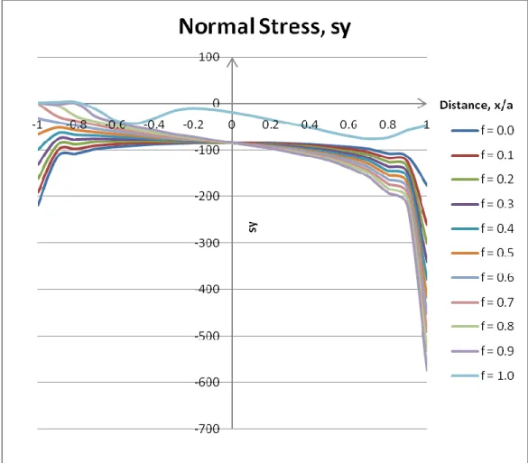
Figure 4.6 Distribution of contact normal stress, sy along the contact interface (f=0.0 until f=1.0)
4.1.2 Subsurface stress analysis
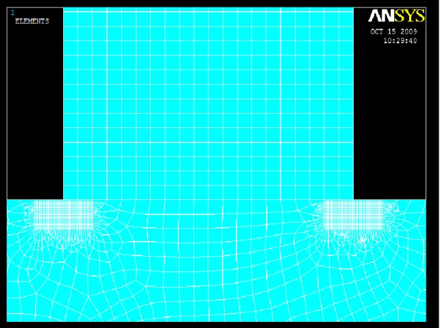
Subsurface stress analysis is carried out in order to determine the stress distribution below the contacting surface focusing at the leading and trailing edge which is at the half plane. Figure 4.7 below shows the location of the subsurface region. Note that the concerned regions have refined elements.
Figure 4.7: Modelling of the subsurface region
As for the subsurface stress analysis, parameters analyzed were normal stress, σ and shear stress, τ only. In addition, only three values of coefficient of friction, f = 0.2, 0.4, and 0.8 were used. Contour plots were utilized to represent the distribution of stresses beneath the contact interface and were shown in the figures below.
4.1.3 Subsurface stress distribution for f = 0.2
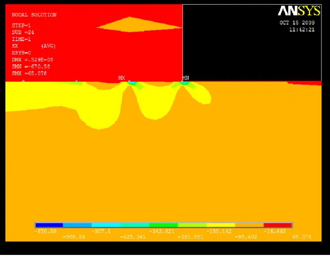
Figure 4.8: Contour plot of normal stress distribution in X-direction (leading edge; f = 0.2)
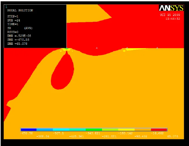
Figure 4.9: Contour plot of normal stress distribution in X-direction (trailing edge; f = 0.2)
Figure 4.10: Contour plot of normal stress distribution in Y-direction (leading edge; f = 0.2)
Figure 4.11: Contour plot of normal stress distribution in X-direction (trailing edge; f = 0.2)
Figure 4.12: Contour plot of shear stress distribution in XY-direction (leading edge; f = 0.2)
Figure 4.13: Contour plot of shear stress distribution in XY-direction (trailing edge; f = 0.2)
4.1.4 Subsurface Stress Distribution for f = 0.4
Figure 4.14: Contour plot of normal stress distribution in X-direction (leading edge; f = 0.4)
Figure 4.15: Contour plot of normal stress distribution in X-direction (trailing edge; f = 0.4)
Figure 4.16: Contour plot of normal stress distribution in Y-direction (leading edge; f = 0.4)
Figure 4.17: Contour plot of normal stress distribution in Y-direction (trailing edge; f = 0.4)
Figure 4.18: Contour plot of shear stress distribution in XY-direction (leading edge; f = 0.4)
Figure 4.19: Contour plot of shear stress distribution in XY-direction (trailing edge; f = 0.4)
4.1.5 Subsurface Stress Distribution for f = 0.8
Figure 4.20: Contour plot of normal stress distribution in X-direction
(leading edge; f = 0.8)
Figure 4.21: Contour plot of normal stress distribution in X-direction (trailing edge; f = 0.8)
Figure 4.22: Contour plot of normal stress distribution in Y-direction (leading edge; f = 0.8)
Figure 4.23: Contour plot of normal stress distribution in Y-direction (trailing edge; f = 0.8)
Figure 4.24: Contour plot of shear stress distribution in XY-direction (trailing edge; f = 0.8)
CHAPTER 5
CONCLUSION AND RECOMMENDATION
5.0 Conclusion
Based on the results of the contact analysis using ANSYS, it can be concluded that the solution of the contact at its leading edge, and trailing edge which is represented by the graphs, show that the contact pressure and stress in Y-direction, have high values compared to the other point along the contact interface. This shows that two bodies having the same modulus of elasticity in contact and been given pressure on the square punch exhibit higher contact pressure and stress at the edge compared to the interior points between the leading and trailing edge.
But, for certain cases, the stress values at the trailing edge are lower than the center of the contact interface, this is probably because the square punch was slightly uplifted when the shearing force, q is applied to make it slide, thus, making the contact at that area not completely touched.
After analyzing the results, it can be concluded that these phenomena satisfy the theory of contacts between two bodies which are both elastically similar in which it stated that the contact pressure and stress distribution adjacent to the to the edge is significant influenced by the coefficient of friction [1].
Further analysis was carried out in order to find the sub-surface stresses just below the contact interface. It was found that, coefficient of friction, f also affecting the value of stress. Higher f, gives higher value of stress at the leading edge.
5.1 RECOMMENDATION
There is suggestion in order to make this analysis more precise which is comparing results of the analysis using Finite Element Method software, ANSYS with the analytical method.
In order to improve the results of the analysis, recommendations for future analysis for this project is refining the meshing on the interface between the square punch and the half plane to get more precise value of the contact pressure and contact frictional stresses.
REFERENCES
[1] Saravanan Karuppanan, Churchman, C.H, and Hills, D.A, 2008, “Sliding frictional contact between a square block and an elastically similar half-plane,” European Journal of Mechanics A/Solids 27: 443-459.
[2] Churchman, C.H, and Hills, D.A, 2008, “Asymptotic results for slipping complete Frictional contacts,” European Journal of Mechanics A/Solids 22: 793-800.
[3] Johnson K.L 1985, Contact Mechanics, Cambridge, Cambridge University Press.
[4] Seshu P. 2006, Textbook of Finite Element Analysis, New Delhi, Prentice Hall of India Private Limited.
[5] Y.J Xie, D.A Hills, 2003, “Crack Initiation at Contact Surface,” Theoretical and Applied Fracture Mechanics 40: 279-283.