ISSN 0127-9386 (Online)
http://dx.doi.org/10.24200/jonus.vol8iss3pp177-208
A HISTORICAL PERSPECTIVE OF TRADE LIBERALISATION DYNAMICS IN BANGLADESH: IMPACTS OF NATURAL CALAMITY RISK, GROSS DOMESTIC
PRODUCT, FOREIGN EXCHANGE RESERVE, RELATIVE PRICE AND TARIFF ON IMPORT DEMAND
1Husne Ara Shikha, *2Md. Mahmudul Alam, 3Md. Wahid Murad, *4Jamaliah Said & 5Zafar U. Ahmed
1 The Central Bank of Bangladesh, Dhaka, Bangladesh.
2 Economic and Financial Policy Institute, School of Economics, Finance and Banking, Universiti Utara Malaysia Sintok, 06010 Kedah, Malaysia.
3 UniSA College, University of South Australia, Adelaide, Australia.
2,4 Accounting Research Institute, Universiti Teknologi MARA, 40450 Shah Alam, Malaysia.
5 School of Business, Thu Dau Mot University, Thu Dau Mot City, Bình Dương Province, Vietnam.
*Corresponding author: [email protected] / [email protected]
Received: 15.05.2023 Accepted: 17.08.2023
ABSTRACT
Purpose: After the trade liberation, Bangladesh has faced the crisis of trade imbalance. Therefore, trade liberation is considered as the driving force behind the crisis. To investigate this historical allegation, this study aims at analysing the factors that determined the post trade liberalisation aggregate import demand function of Bangladesh.
Design/Methodology/Approach: Based on quarterly data from trade liberalisation period to reaching the economic stability period, 1992Q1 - 2007Q4, an autoregressive distributed lag (ARDL) approach to cointegration and an error correction model (ECM) have been utilised to estimate the impacts of natural calamity, gross domestic product, foreign exchange reserve, relative price and tariff on
Findings: Empirical results revealed that the natural calamity is identified to be nonresponsive to the nation's aggregate import demand both in the short and long run. This indicates that Bangladesh can meet the natural crisis related demand by herself without influencing its aggregate import demand.
Results also revealed that the import volume of Bangladesh is cointegrated with relative import price, actual GDP and real foreign exchange reserve of the country. The import demand of the country can largely be described by its real GDP, while it is found inversely associated with relative price ratio in the long run. The long run association among import demand and tariff rate indicates that trade liberalisation has a significant positive impact on the country's aggregate import demand, as well as real foreign exchange reserve, as explained by the reduction in tariff rate.
Research Implication: Developing countries like Bangladesh and the relevant business stakeholders would have considerable implications of such empirical findings with their trade policies, particularly how they should respond to unpredictable scenarios caused by the factors such as natural calamity, foreign exchange reserve, tariff, etc.
Originality Value: The originality of the study lies in its uniqueness in using the historical data and factors that no studies have so far used in analysing the import demand function of Bangladesh.
Keywords: Natural calamity, import demand, foreign exchange reserve, gross domestic product, tariff, trade liberalisation, Bangladesh.
Cite as: Shikha, H. A., Alam, M. M., Murad, M. W., Said, J., & Ahmed, Z. U. (2023). A historical perspective of trade liberalisation dynamics in Bangladesh: impacts of natural calamity risk, gross domestic product, foreign exchange reserve, relative price and tariff on import demand. Journal of Nusantara Studies, 8(3), 177-208. http://dx.doi.org/10.24200/jonus.vol8iss3pp177-208
1.0 INTRODUCTION
Bangladesh has struggled with a persistent import/export shortfall and a stunted GDP growth rate since its independence in 1971. In this context, trade liberalisation became one of the most pressing policy issues for countries across the world, predominantly in developing nations, in the mid-1980s. During the time frame, Bangladesh adopted a highly regulated trade system approach. Strong levies and non-levy trade barriers, as well as an artificially inflated exchange rate framework, were all part of the government's import-substitution industrialization policy.
This approach was sought with the aims of improving the country's payment balance and
establishing a stable homegrown market for assembling businesses (Bhuyan & Rashid, 1993).
When a moderate liberalisation arrangement was established in the 1980s, the trade system took a major step forward. For instance, Bangladesh's import payments in 1973-74 were just 8.77 percent of its actual Gross Domestic Product (GDP) at 1972-73 rates. It then erupted, hitting 30.5 percent of GDP in 1986-87. Export income on the other hand represented for 5.69 percent of GDP in 1973-74, but it grew to 21.8 percent of GDP in 1986-87.
Given the present circumstance, Bangladesh, a developing emerging country, has been drastically changing its trade system since 1992, establishing quite possibly the most extensive economic strategy system changes ever. Bangladesh is expected to accomplish higher trade growth via improved resource distribution and technological innovation, higher economic broadening, reviving sustainable import replacement, and limit non-essential imports to avoid balance-of-payment and balance-of-trade issues, as a result of liberalisation (Ahmed, 2001). However, various elements are crucial to understand during the period 1992-1996, when trade liberalisation was intensified. The first move was to keep CPI inflation under control. Second, the fiscal debt was minimised. Third, the current account arrears were diminished. Fourth, because of increased domestic resource assembly as a result of tax changes, dependence on international assistance has decreased significantly. Fifth, Bangladesh was able to attain macroeconomic strength during this period without slowing down its investment and growth rates. In reality, whether trade will function as a growth engine or not is strongly reliant on the responsiveness of price and returns of an economy's exports and imports (Alam et al., 2009; Uddin et al., 2010). Johnson (1958) demonstrated that in a two- nation model with comparable income and price growth rates, when one of the states' revenue elasticity of demand differs from that of its trading associate, it is likely for the state's balance of payments to shrink compared to its trading nation. Furthermore, the Mershal Learner concept recognizes that the intensity of trade harmony is largely determined by the scale of price elasticity of imports and exports. Besides that, it is a well-known reality that the efficacy of global trade approaches is strongly reliant on trade (export and import income and price) flexibility (Murray & Ginman, 1976).
Through specialisation and technical advancements, trade liberalisation is thought to improve trade efficiency and financial growth (Hoque & Yusop, 2010, 2012). As per to Ernst (2005), the influence of trade openness in Argentina and Brazil was unappealing; nevertheless, profit and work in the assembly region improved in the case of Mexico in late 1990s. According
to Fu and Balasubramanyam (2005), exports in China have a positive and significant effect on jobs. On the other hand, a number of studies have discovered negative associations between trade transition and jobs. For instance, in the late 1970s and early 1980s, Uruguay (1994) discovered that trade liberalisation had a detrimental effect on jobs. Greenaway et al. (1998) discovered that the manufacturing industry in the country suffered significant job losses.
Brazil, Carneiro and Arbache (2003) also discovered that trade advancement had only a marginal effect on macroeconomic conditions and job market measures.
Nonetheless, during the pre-liberalisation period (1972-1973 to 1990-1991), Bangladesh's import/export imbalance expanded from US$1.45 billion to US$2.45 billion between 1985 and 1991, with a normal import/export imbalance of 6.90 percent of GDP (Hoque & Yusop, 2012). While the GDP increased from $15.58 billion to $30.98 billion for the same time span, the overall annual growth rate was less than 5% in absolute terms (IFS of IMF). In comparison, the development phase of a couple of East Asian nations with which Bangladesh has a long-standing cultural and trade partnership was extremely poor. Now that trade liberalisation strategies have been applied for more than a decade, certain effects on GDP growth and trade equilibrium must be observed. In the post-liberalisation phase, the normal GDP growth rate was slightly higher than 5%. Moreover, imports were becoming quicker than exports, thus expanding the import/export imbalance. The standard import/export imbalance as a proportion of GDP has improved to 6.97 percent, up from 6.90 percent prior to liberalisation (Hoque & Yusop, 2012). This implies that trade reforms aren't accomplishing the objective of resolving trade irregularities. Instead, the usual import/export imbalance as a proportion of GDP is escalating, causing worries in Bangladesh. One might contend that trade liberalisation is a driving force behind these opposing trends. Bangladesh's internal economic irregularities, according to the World Bank (WB), are to blame for the trade imbalance crisis. In light of this, empirical research on aggregate import demand function of Bangladesh with a focus on after the trade liberalisation scenario is much needed.
Therefore, the objective of the study is to investigate the factors that determined the import demand function of Bangladesh from the historical perspective from trade liberalisation period to reaching the economic stability period. With a view to achieving this objective, the impact of trade liberalisation was examined using tariff rate as an explanatory feature. Other important factors such as natural calamity, GDP, foreign exchange reserve and relative price are also considered to explain the country's import demand function. This study will benefit
the researchers and policy makers to assess the post-trade liberalisation situation while understanding the historical claim of the initial trade liberalisation imbalance crisis of Bangladesh.
2.0 LITERATURE REVIEW
The studies for both developed and developing nations on import demand function have been considered by plentiful authors such as Babatunde and Egwaikhide (2010), Hye and Mashkoor (2010), Narayan and Narayan (2010), Omotor (2010), Modeste (2011), Nwogwugwu et al.
(2015), and Mugableh (2017). The import demand function is explained by a variety of non- economic and economic features. In this paper, we review the most recent research in an attempt to identify the most suitable variables for studying the import demand function.
The income elasticities of imports and exports and its aggregate price have been thoroughly studied for numerous countries over the decades. There have been some earlier impressive empirical studies that investigated the relationship among imports, import prices and related variables (Carone, 1996; Reinhart, 1995). Murray and Ginman (1976) investigated the overall import demand using 15 years of US export and import results.
According to their results, import price elasticity varied from 0.71 to 1.05, while income elasticity extended from 0.96 to 1.94. Similarly, using cointegration and error correction approaches, Carone (1996) investigated the U.S. import demand with the data of 23 years (1970 to 1992), and found statistically significant association among real income and relative prices and the demand function of import. The difference of income elasticity from developed to developing countries was observed in a study of Reinhart (1995). Johansen cointegration and the techniques of dynamic estimator (Stock & Watson, 1988) were used to data of 12 developing countries for estimating structural import demand functions.
Siddique (1997) used a log-linear model to project the demand equation for Indonesia for the period of 1971-1993. He found income to be a crucial determinant of import demand in Indonesia and estimated an import demand of 1.91 income elasticity. He also estimated the aggregate imports for Indonesia for the period of 1971-1993. The income elasticity of demand for import was found to be significantly higher than one, suggesting that imports are income elastic in Indonesia. As Indonesia’s economy grows, imports will grow at a higher rate. The price elasticity of Indonesian imports, on the other hand, was discovered to be less than one in numerical value suggesting the price inelastic import demand in Indonesia.
Using fully modified ordinary least squares (FMOLS) with cointegration technique, Senhadji (1998) investigated systematic import demand functions for 77 nations. The results indicated that the income and price elasticities for short run was found to be -0.26 and 0.45 in the case of import demand, while for long run, it was found to be -1.08 and 1.45 correspondingly. In a similar fashion, the import demand function for Thailand was also derived by Mah (1999) which considers relative price and real income. The results were found to be insignificant and smaller income elasticity was found to be 1.4 to 1.7. However, an interesting finding reported in his study is that import demand increases after liberalising trade in Thailand. To delve into depth about the nature of import demand and income elasticity, likewise, Aydin et al. (2004) also estimated the import demand function using a vector autoregressive model for the case of Turkey. The results are profoundly comparable between long and short run scenarios. For instance, the import demand's long-run income and price elasticity was found to be very high (e.g., 1.99 and 0.402 respectively), while the short run was found to be 0.366 and -0.509, indicating that price and income elasticity for import demand is higher for long run in Turkish economy.
The effect of trade liberalisation on selected macro-economic indicators was examined by Santos-Paulio and Thirlwall (2004). Using generalised methods of moment (GMM) with fixed effects technique and data from 22 developing countries, their study revealed that export growth was smaller than import growth, while considering the trade liberalisation. In the same study, they also summarised that the increase of income elasticity for import and export demand was almost equal. However, the variation was observed in import price elasticity and export demand, where import price elasticity of demand upturn rather than its counter export demand.
Conclusively, they came up with the summary with evidence that trade liberalisation does not help increase the balance of trade position.
The extent of trade liberalisation impact on import volume for the Mexican economy was examined by Lopez (2005), using the estimation method of autoregressive distributed lag (ARDL). In the long run, the study discovered that the price and income elasticity of the import demand function were reported to be substantially significant. In addition, the error correction coefficients were also found to be statistically significant, suggesting that trade liberalisation has a positive influence on the development of imports in the case of the Mexican economy.
Nguyen and Bhuiyan (1977) examined the income and price elasticity of demand for imports in Southeast Asian nations like India, Pakistan, Bangladesh and Sri Lanka. Their findings
indicated that the income and price elasticity of demand for imports were positively significant and greater than one which was only for two categories of import goods; however, for other goods it was price inelastic. Likewise, Ju et al. (2010) conducted a study considering sizable samples from developing countries to observe the influence of trade liberalisation on import and how inward trade increases with lowering tariff. The results accentuated that liberalisation of trade disproportionately increased the volume of trade inflow and outflow among these countries. Using the same Johansen process, in the import demand function, Dutta and Ahmed (2004) discovered an indication of a long-run association. They also included a dummy variable for the trade progression era in the model (1992–1995). The analysis, however, got the relative price elasticity wrong (0.37) and had an exceptionally low coefficient of pay flexibility (0.03). Income and price elasticity in the short run were identified to be 1.48 and 0.47, respectively. Subsequently, import advancement didn't appear to fundamentally affect import demand.
In the case of the Bangladesh economy, several studies have been carried out to analyse the import demand role. For instance, a study of Hossain (2013) explored the behaviour of import demand, considering 34 years of macro-economic data which explain import and export of the country. The ARDL estimation confirmed the existence of normal behaved import demand function, explaining the no evidence of disturbance in economic stability due to trade liberalisation. Similarly, another past study investigated the influence of trade liberalisation on Bangladeshi import demand (see for details, Hoque & Yusop, 2010). The ARDL Bound Test technique confirmed that the total import increased manifold in the short run, due to a lowering import duty. However, for the long run it was insignificant. More specifically, this study advocated that in the long run, trade liberalisation with adopting no-tariff measures had minimal positive effect on the total import demand. At the same time, the study concluded that reducing tariffs increases imports to some degree and to some extent and; therefore, enhances trade balance, while without trade liberalisation, a rise in the income upsurges imports considerably and later deteriorates the trade balance.
Another study by Hussain (2004) predicted the differentiated and aggregated import demand functions for Bangladesh's economy from 1973 to 2000 for import products. Ordinary Least Square method was applied to measure the equation of linear and log-linear demand for import. As expected, the demand elasticity of income for all commodities excluding rice and wheat was found to be positive. Nearly all the coefficients of income were found to be
statistically substantial. The coefficients of relative import prices were found to range from - 1.66 to -0.73. The relative price coefficients of imported soya bean oil and rice, on the other hand, were negative and statistically insignificant. Islam and Hassan (2004) used quarterly time series and Johansen–Juselius' multivariate cointegration method to empirically estimate a number of useful factors of the total demand function for import in Bangladesh. Their cointegration results showed that relative prices and incomes dominate the demand role for imports in Bangladesh. The findings also indicate that the income elasticity of demand for import is higher than one significantly. This demonstrates that imports as a whole are considered as "luxury" products. The relative import price's effect was found to be strongly negative; however, it had an elasticity coefficient that was less than one.
There were also some other studies conducted looking into aggregate import demand and export demand function for Bangladesh. Kabir (1988) studied to evaluate the aggregate demand functions for import and export for Bangladesh, taking into account the relative import prices, foreign exchange reserves, real per capita income (GDP), exchange rate, and foreign aids as descriptive factors. In his estimation, he used the quarterly data for the year 1973 to 1983. Bangladesh's projected income elasticity of import demand had the expected positive sign with coefficient greater than one, and it was found to have reached a statistical level of significance of 5. The estimated relative import price elasticity was negative, as expected. In the final analysis, Kabir (1988) found foreign aid, international reserve and foreign price measured in the US dollar to be statistically significant. Meanwhile, Shilpi (1990) used the OLS technique and annual data from 1972 to 1987 to measure the demand for imports in Bangladesh based on income and price elasticities. The author also used relative import price, foreign exchange reserve, GDP, and a dummy as descriptive factor. He discovered that the income elasticity of import in all of the estimated functions was positive, and that it was statistically significant at the 5% level in all equations except the ones for rice and cotton. The estimated coefficients were insignificant in both cases, and only in one case, raw cotton, did the income elasticity of import demand drop below one. In all other cases, import demand was found to be elastic in terms of income. On the contrary, the coefficient of relative import price does not appear to be statistically significant for all cases. All the equations had good fit as apparent from their estimated R2 values. However, the major findings of the Shilpi’s (1990) study are that while import demand for Bangladesh is price inelastic, it is actually income elastic.
Furthermore, from 1974 to 1994, Dutta and Ahmed (1999) utilised the error correction and cointegration approach to assess demand function for imports in Bangladesh in the long run.
In this regard, for measuring demand functions, the study considered two sort of variables. For the first one, the actual importation price and the actual GDP were considered, and for the second model, not only the actual real GDP and import prices, but also the actual imports and another dummy factor were taken. This dummy descriptive variable was used to demonstrate the effect of import liberalisation. They discovered only a single relationship that cointegrates the import price, GDP and real forex reserves. As the error correction coefficient for the first model was found negative and achieved statistical level of significance, it specifies that the variables' long-run equilibrium is valid. In the case of the second model, the coefficients of variables considered were found to be statistically significant as well. Like the first model, the projected error correction was found to have achieved statistical significance with an anticipated negative sign, which also affirms association between the factors in the long-run equilibrium. However, since the dummy variable's coefficients were significantly lower in each of these models, it can be ascribed that the liberalisation of trade policies was not completely functional.
On the other hand, global trade is highly prone to natural disasters due to its dependence on trade and transportation infrastructure. For instance, Gassebner et al. (2010) discovered that a major catastrophe lowers imports by 0.2 percent on average, putting a boundary condition on a country's degree of democracy. Meanwhile, Oh and Reuveny (2010) differentiate between climatic and geophysical events, observing that an extra climatic event decreases imports by 2.68 percent. On the supply side, climate events can devastate vital trade highways and ports, limiting a nation's capacity to export efficiently. The destruction of public and private assets (e.g., energy plants, industries) that are critical for production also has an impact on export capability. The loss of resources behaves as a negative income signal on the consumer side;
non-insured households will also have to spend a portion of their budget on non-tradable facilities to fix their homes. Imports into the affected nation are reduced by both methods.
Natural disasters can also disrupt existing trading relationships with customers. Supply chains for intermediate inputs and services could be disrupted (De Mel et al., 2012), resulting in lower imports or companies having to source inputs from various suppliers, most likely from abroad, to compensate for the damaged infrastructure buildings.
Narayan and Narayan (2010) used two cointegration methods for South Africa and Mauritius to re-estimate the import demand elasticities. Both nations' long-run elasticities were examined utilising the ARDL method and yearly time arrangement data from 1960 to 1996 for South Africa and 1963 to 1995 for Mauritius. Over time, the two strategies discovered reliable outcomes and revealed a strong link among import volumes, relative costs, and local income, with local income generally influencing import volumes. The findings revealed that import volumes were pushed eight years (South Africa) and three years (Mauritius) away from usual levels after a disruption to the import demand model. Alias et al. (2001) assessed the long-run connection among expenditure components and total imports of 5-ASEAN (Indonesia, Singapore, Malaysia, Thailand and The Philippines). The author used the Johansen multivariate co-joining examination. With the exception of Singapore, the report used annual data from 1968 to 1998 for four Asian nations (1974-1998). Imports, investment spending, consumption expenses, relative price, exports, and the nation's capacity to generate and supply merchandise were all included in the study. The findings show that import demand and its contributing factors are linked in Asian nations. In the case of Caribbean and Latin American nations, Ozturk and Acaravci (2009) discovered that the amount of import demand was negatively associated with relative costs and positively associated with real income.
The influence of import levy as a variable exchange rate is studied in some literature.
Yu (2015) examined the influence of lower tariffs on materials and manufactured imported goods on the efficiency of big trading companies in China. Similarly, Brandt et al. (2017) explored the impact of the levy reduction following the entrance of China into the WTO on manufacturing corporations' performance. Liu et al. (2019) investigated the influence of trade liberalisation on local vertical integration utilising acceptance of China to the World Trade Organization (WTO) like a semi-regular case study. According to Hoque and Yusop (2010), trade liberalisation by lowering import tariffs increases total imports for the time being, but has a major long-term effect. In the long run, trade liberalisation based on improving the non-levy system has substantial but more negative effects on total imports. Mah (2000) further conducted a study on Korean products labelling information technology (IT). The income elasticity of import demand in the long run and price of the IT products were then tested by utilising an unobstructed error correction test which produced robust outcomes, indicating the lessening tariff rate would induce the import of related IT goods significantly. The similar conclusion was also drawn by Mehta and Parikh (2005), when they studied both developed and
developing countries. Their results also support that trade liberalisation with lowering tariffs incline the price elasticity of import demand for selected commodities. Santos-Paulino (2002) studied the relationship of tariff rates and non-tax trade hindrance reduction on imports from 22 developing countries. The effect of macroeconomic factors on import growth is determined using a Dynamic Panel Data analysis procedure on yearly data between 1976 to 1998.
Empirical outcomes discovered a critical positive association of price level, local income, and disposal of trade strategy alteration with import development, despite the fact that import obligations have significant negative effects.
Nigeria's empirical investigation yielded astonishing results. Chimobi and Ogbonna (2008), for example, used cointegration and blunder adjustment model methodologies to examine the behaviour of Nigeria's total imports from 1980 to 2005. They discovered that the role of import demand in Nigeria was mainly clarified by actual GDP to a great extent.
Babatunde and Egwaikhide (2010) used a limit checking methodology to look at total import demand behaviour in Nigeria from 1980 to 2006. Imports, relative prices, and income were found to be cointegrated, with long-run elasticities of import demand for relative prices and income of - 0.133 and 2.48, respectively. The findings proposed that the Marshall-Lerner requirements haven’t been met in Nigeria because the price elasticity of demand for imports is not as high as others. Omoke (2010) also used a blunder-correction technique and cointegration methods to look at the Nigerian import demand feature. Despite the fact that there was no cointegration among the variables, the results showed that the evaluations were statistically significant, suggesting there was no long-term association among them. The findings also revealed that actual GDP to be one of the main contributing factors on import demand in Nigeria, and in the short term, it has a positive influence on the number of imports. Finally, Fatukasi and Awomuse (2011) used data from 1970 to 2008 to observe the factors that influence the demand function for imports in Nigeria. In the short run, actual GDP was a key contributing factor of Nigeria’s import demand, according to the findings of the report, which used an error correction model methodology. The outcome additionally displayed the presence of a long-run association between the factors.
Omoke (2010) also examined the import demand function for Nigeria utilising cointegration strategies and the error amendment method. Even though the variable failed to show any cointegration, the results showed that the evaluations were statistically significant, implying that there was no association among the variables in the long-run. The findings have
identified relative price as a contributing factor in the import demand function, which has a positive effect on the volume of imports in Nigeria. Emran and Shilpi (2010) created an underlying import demand model for India by including a compulsory foreign exchange restriction. The authors used three different econometric methods to determine import demand elasticities over time, namely FM-AADL (Fully Modified Augmented ADL), ARDL and DOLS. Import value elasticities increased from 0.63 to 0.79, according to the findings. Sultan (2011) used Johansen's cointegration technique to create an association between foreign reserve, import demand, wages, and relative prices in the long run. Arize and Malindretos (2012) discovered cointegration among these variables using four elective co-integration strategies and quarterly data gathering. None of these studies, however, consider how import demand is influenced by import liberalisation. The import demand feature was evaluated by Nell (2013) using ARDL Model. For India's post-liberalization era, the author obtained a strong level of income elasticity of imports (2.38) for goods and services. This may be because of the foreign exchange reserve factor was removed from the model. Furthermore, the price elasticity measure is both positive and insignificant, which is hypothetically conflicting. Narayan and Narayan (2005) investigated import demand behaviour of Fiji from 1970-2000 using a disaggregated import demand feature. The author presented relevant factors such as relative price, investment expenditure, export expenditure and total consumption using (ARDL) model to estimate Fiji's import demand feature. The discovers outline that import demand and independent variables such as relative price have a long-term association.
In their study of Pakistan's import demand, Arize et al. (2004) discovered that import demand and real foreign reserves have a long-term association. Moreover, the authors also found an important long-run positive relationship among the same variables, but reached the conclusion that the result is statistically insignificant in the short run. Arize and Osang (2007) observe that actual foreign reserves have an influence on import size, both long- and short-term in seven central American nations, with an elasticity of about one-quarter. Additionally, the findings demonstrate that the actual foreign reserves coefficient is significantly positive.
Sultan's (2011) study has provided additional empirical evidence on the influence of actual foreign exchange reserves on real imports. His analyses, based on India's annual data, reveal a truly enormous reaction of real imports to variations in actual foreign exchange reserves. The author also demonstrates that both in the short and long run, the actual foreign reserves have a significant positive influence on real imports. Aziz (2013) focused on the total import demand
function for developing countries, using Bangladesh as an example. He used the error correction mechanism and a few co-integration evaluation procedures. The findings show that in both the short and long term, real wages, relative import prices, foreign exchange reserves, and export demand are statistically significant. As a consequence, the accessibility of adequate foreign exchange reserves may likewise be a major factor of non-industrial nations' import demand. Understandably, exporters are unlikely to be interested in supplying their goods to a nation that isn't willing to pay its foreign duties. A nation's adequate foreign exchange reserves will serve as an assurance of its capacity to settle for import charges. In this way, a growing body of literature (like Arize & Osang, 2007; Emran & Shilpi, 2001) suggest that "foreign exchange reserves" is one of the contributing factors to underdeveloped nations' import demand. As a consequence, the import demand position is estimated in this study, with one of the causal factors being foreign exchange reserves. It's worth noting that since the mid- 1980s, trade liberalisation has been a major policy priority for Bangladesh.
3.0 METHODOLOGY 3.1 Data and Variables
To achieve a deeper understanding of post-trade liberalisation dynamics, particularly the historical perspective of imports in Bangladesh, this study utilised quarterly time series data from 1992Q1 to 2007Q4, which covers the timeframe from the trade liberalisation time to reaching the economic stability period in Bangladesh. This study considered data up to 2007, because the current ruling party – Bangladesh Awami League – has been running the government since 2008, which is considered as a structural change with stability in the political and macroeconomic factors.
All variables were given their nominal values (in local currency), while GDP and foreign exchange reserves were given their original values. Many of the variables were subjected to natural logarithms. Finally, data on import volumes, foreign exchange reserves, relative costs, and tariff rates were plotted to see if there is any seasonality. Further explanations of all the variables are provided below:
● Natural Calamity (DN): Natural calamity was used as a dummy explanatory component. When there is a natural calamity, the variable is set to 1, and when there isn't, it is set to 0. The information was gathered from the International Seminar on Natural Hazards Monitoring Proceedings, which was held on 7-11 January 2002 in Karachi, Pakistan, and was organised by Inter Islamic Network on Space Science and Technology.
● Import Volume (M): Import demand is measured by the aggregate import volume expressed in local currency. The information is gathered from various data sources published monthly by Bangladesh Bank, the country's central bank.
● Relative Price of Imports (RP) (1990=100): The information is based on the import directory (1990=100), deflated by local rates (CPI) (1990=100). The CPI and The IFS database is utilised to establish the import value index.
● Real Gross Domestic Product (Y): IFS provides GDP records at predetermined rates for the year 2000. Due to the lack of quarterly actual GDP data, from annual data, the quarterly GDP data was produced using E-Views software (Dutta & Ahmed, 1999).
Figure 1 depicts the pattern of yearly and quarterly real GDP results.
Figure 1: a. RGDP data (Quarterly) b. RGDP data (in yearly)
● Real Foreign Exchange Reserve (RR): To acquire actual foreign exchange reserves, the CPI was used to deflate nominal foreign exchange reserves. The information on foreign exchange reserves comes from a number of Bangladesh Bank reports. The foreign Exchange reserve that was used in the study is the starting date data for each quarter.
● Tariff Rate (TR): The study determined to use the average import weighted tariff rate.
Data from the National Board of Revenue was gathered from different issues of Bangladesh's Annual Economic Review. The difficulty of determining the degree of outward or inward orientation is an issue that all empirical studies deal with. The justification for this is that the actual rate of defence is determined by a complicated
combination of tariffs, quotas, exchange rate limits, and a slew of other regulatory stumbling blocks. The assessment of trade liberalisation could be determined whichever occurrence or outcome (Ahmed, 2001). While indicators such as the trade- to-GDP ratio and the import concentration ratio derive data about policy-induced barriers to trade from factors that could influence import costs or trade flows, the prevalence of trade policy tools is a different story (like average import tariff collection rate, black market premium, index of effective rate of protection, actual effective exchange rate), and can; likewise, be utilised as a measurement of trade liberalisation.
Nevertheless, the average import duty is utilised as a metric of trade liberalisation in this study. As an indicator of trade liberalisation, the average import duty rate has many benefits (Ghani & Jayarajah, 1995): (i) It is an imperative factor of the degree of import protection; (ii) In contrast to metrics focused on trade flows (such as the GDP/export ratio), Tariff rates are a strong measure of trade strategy; and (iii) the tariff rate is unaffected by the arbitrary existence of the indexes.
3.2 Econometric Modelling
The standard approaches for analysing non-stationary time series are Engle & Granger and Johansen's cointegration test. This co-integration test eliminates multivariate analysis since Engle and Granger's co-integration is a bi-variant technique. The deficiency of the method associates with Ordinary Least Square (OLS) method while measuring relationship of long-run equilibrium as the Engle & Granger’s co integration only take the form of non-stationary variables. Application of this technique is debatable as it produces significant biases by omitting the dynamics, and thus jeopardises the estimator's efficiency. Johansen’s method is different from Engle & Granger’s as the approach integrates omitted lagged variables into the estimation process to reduce bias. Nevertheless, Johansen co-integration technique is criticised due to sensitivity while including lag values during test procedure (Gonzalo, 1994).
Furthermore, the technique yields many co-integrating vectors which lead complexity in interpreting economic relationships for the most expected significant vector (Ang, 2009).
Overall, both the Johansen and Engle-Granger approaches failed to explicate their critics especially for the ground validity, i.e., these approaches are only valid for the same order of integration. Practically, however, these techniques generate mixed order of integration during the regression procedure which is not desirable.
Upon considering the above facts, the Autoregressive Distributed Lag (ARDL) method is utilised in this study to investigate the relationship in the long run under changing key variables scenarios. The ARDL has some key distinctive features: (1) the ARDL approach use Ordinary Least Square (OLS) for estimating co-integration relationship which is done by selecting respective lag order from the model considered; (2) this technique is found to be statistically significant for all types of variables with I(1), I(0) or jointly co-integrated nature, warranting not to opt for unit root test, and (3) When the model includes an I(2) series, the approach directs a way. The approach directs a way when the I(2) sequence is present inside the framework of the model.
3.2.1 Model Specification
According to the studies conducted by Ang and McKibbin (2005), Khan et al. (2005), Fosu and Magnus (2006), the vector error correction model (VECM), and the ARDL version can be described as follows:
∆= 𝛽0+𝛽1+𝛽2𝐿𝑌 𝑡−1+ 𝛽3𝐿𝑅𝑃𝑡−1+ 𝛽3 𝐿𝑅𝑅𝑡−1+ 𝛽4𝐿𝑇𝑅𝑡−1+ 𝛽5𝐷𝑁𝑡−1+
∑𝑝𝑖=1 𝛾∆ + ∑𝑞𝑗=1 𝛿𝑗∆ 𝑖 + ∑𝑞𝑘 𝜛𝑘𝛥𝐿𝑅𝑃𝑡−𝑘+ ∑𝑞𝑙=1 𝜑𝑙∆𝐿𝑅𝑅𝑡−𝑙+
∑𝑞𝑚=1 𝜂𝑚+𝜀𝑡 (1)
3.2.2 Estimation Procedure
Firstly, this study assessed equation (1) by applying OLS method and later the Wald Test (F- test) was utilised in this analysis for combined implication of coefficients of lagged variables to see whether there was a long-run association between the factors. The null hypothesis against the alternative hypothesis will reveal whether there is no cointegration amongst the variables.
As per Pesaran et al. (2001), the significance of the F- test is also linked to the critical value of both the lower and upper bound. The null hypothesis would be accepted if the F-test value is less than the lower critical value, implying that there is no co-integration between the factors.
Meanwhile, the null hypothesis of no cointegration is dismissed. If the F-test value is greater than the upper critical value, it implies that the variables have a long-term association. And, if the value of F-test exists in the middle of the critical upper and lower values, the examination is considered to be equivocal. In the subsequent phase, after the establishment of a co
integration association between the variables, co integration relationship among the factors, and the long-run coefficient of the ARDL model can be measured as:
= 𝛽0+ ∑𝑝𝑖=1 𝛾𝑖 𝐿𝑀𝑡−𝑖∑𝑞1𝑗=0 𝛿𝑗𝑙𝑛 𝑙𝑛 𝑌1𝑡−𝑗+ ∑𝑞2𝑙=0 𝜑𝑙𝑙𝑛 𝑙𝑛 𝑅𝑃𝑡−𝑙 + ∑𝑞3𝑚=0 𝜂𝑚
𝑙𝑛 𝑙𝑛 𝑅𝑅𝑡−𝑚+ ∑𝑞4𝑚=0 𝜂𝑚+𝜀𝑡 (2)
During this process, SIC guidelines were used to decide the acceptable lag time of the ARDL model including all four variables in the analysis. Lastly, the dynamics of the short run were calculated using the error correction model (Equation 3):
∆= 𝛽0+ ∑𝑝𝑖 𝛾𝑖∆ ∑𝑞𝑗 𝛿𝑗∆ 𝑙𝑛 𝑙𝑛 𝑌1𝑡−𝑗+ ∑𝑞𝑙 𝜑𝑙∆ 𝑙𝑛 𝑙𝑛 𝑅𝑃𝑡−𝑙 +
∑𝑞𝑚 𝜂𝑚𝑅𝑅3𝑡−𝑚+ ∑𝑞𝑚=0 𝜂𝑚+ 𝜗𝑒𝑚𝑐𝑡−1+ 𝜀𝑡 (3)
4.0 ANALYSIS AND DISCUSSION 4.1 Descriptive Analysis
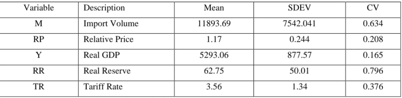
Descriptive statistics such as means, standard deviations (SDEV) and coefficient of variation (CV) for variables like Import Volume, Relative Price, Real GDP, Real Reserve and Tariff Rate from 1992 to 2007 are demonstrated in Table 1.
Table 1: Descriptive statistics of the variables
Variable Description Mean SDEV CV
M Import Volume 11893.69 7542.041 0.634
RP Relative Price 1.17 0.244 0.208
Y Real GDP 5293.06 877.57 0.165
RR Real Reserve 62.75 50.01 0.796
TR Tariff Rate 3.56 1.34 0.376
4.2 Unit Root Test
When performing regression analysis on time series data, it is normal to assume that the selected time series are stationary. The majority of macroeconomic time series are non- stationary, which is validated by empirical evidence, as shown in the serial correlation among consecutive observations, especially when there is a small sampling interval. Therefore, it can
be deduced that the traditional F-tests and t tests are not suitable as they provide confusing outcomes. Studies that fail to justify the existence of unit root non-stationarity could be affected by (i) unauthentic regression issues which is repeatedly considered by a strong R2 and a low Durbin–Watson statistic value (Granger & Newbold, 1974; Phillips, 1987); (ii) Ordinary least squares (OLS) variable estimations are unreliable and inefficient when the factors are co- integrated (Engle & Granger, 1987).
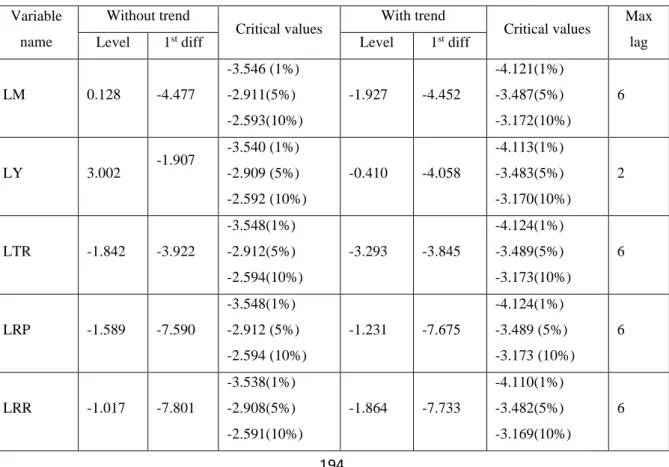
Moreover, the co-integration inspection begins by determining the time series univariate features. The variables must be combined in a precise sequence, and their linear combinations must be stationary, for co-integration to work. There is a feeling that there is no substantive association between the series if they do not combine in the same sequence. If the series are combined in a similar order, it is fair to continue with the co-integration test. The data in this study, on the other hand, is not a stationary and all-time series. Although the existence of unit roots and thus non-stationarity at all levels and the first difference of all variables is verified by Augmented Dickey Fuller (ADF) tests, unit root tests for stationarity are performed at all levels and the first difference of all variables (Table 2), which is the first difference of all variables indicates stationarity. The results of the ADF evaluation are revealed in Table 2.
Table 2: ADF test results
Variable name
Without trend
Critical values With trend
Critical values Max lag
Level 1st diff Level 1st diff
LM 0.128 -4.477
-3.546 (1%) -2.911(5%) -2.593(10%)
-1.927 -4.452
-4.121(1%) -3.487(5%) -3.172(10%)
6
LY 3.002 -1.907 -3.540 (1%) -2.909 (5%) -2.592 (10%)
-0.410 -4.058
-4.113(1%) -3.483(5%) -3.170(10%)
2
LTR -1.842 -3.922
-3.548(1%) -2.912(5%) -2.594(10%)
-3.293 -3.845
-4.124(1%) -3.489(5%) -3.173(10%)
6
LRP -1.589 -7.590
-3.548(1%) -2.912 (5%) -2.594 (10%)
-1.231 -7.675
-4.124(1%) -3.489 (5%) -3.173 (10%)
6
LRR -1.017 -7.801
-3.538(1%) -2.908(5%) -2.591(10%)
-1.864 -7.733
-4.110(1%) -3.482(5%) -3.169(10%)
6
The unit root tests revealed a mixed order of integration, indicating that an ARDL bound evaluation should be used rather than Johansen & Jeslius' or Engle & Granger's approaches.
4.3 Cointegration Analysis
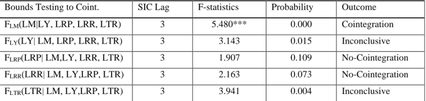
This study estimated equation 1 by following the OLS approach to examine the cointegration relationship. The Wald Test was then used to measure the regressors' combined effect. The estimated F-test (FLM(LM|LY, LRP, LRR, LTR)) is 5.480, which is greater than the critical value of 3.99 (Pesaran et al., 2001). As a consequence, no cointegration is dismissed as a null hypothesis (Table 3). The study discovered through the standardisation procedure that when GDP and tariff rates are viewed as dependent variables, the estimated F-test drops between upper and lower bound of critical values (Pesaran et al., 2001). However, when relative price and real reserve are normalised, the hypothesis of no cointegration is accepted.
Table 3: Bounds test results (Equation 1)
Bounds Testing to Coint. SIC Lag F-statistics Probability Outcome
FLM(LM|LY, LRP, LRR, LTR) 3 5.480*** 0.000 Cointegration
FLY(LY| LM, LRP, LRR, LTR) 3 3.143 0.015 Inconclusive
FLRP(LRP| LM,LY, LRR, LTR) 3 1.907 0.109 No-Cointegration
FLRR(LRR| LM, LY,LRP, LTR) 3 2.163 0.073 No-Cointegration
FLTR(LTR| LM, LY,LRP, LTR) 3 3.941 0.004 Inconclusive
Pesaran et al. (2001) Critical Value at 5% =2.27 3.28 and at 1% = 2.88 3.99
*** denote significant at 1% level
4.4 Long-Run Findings
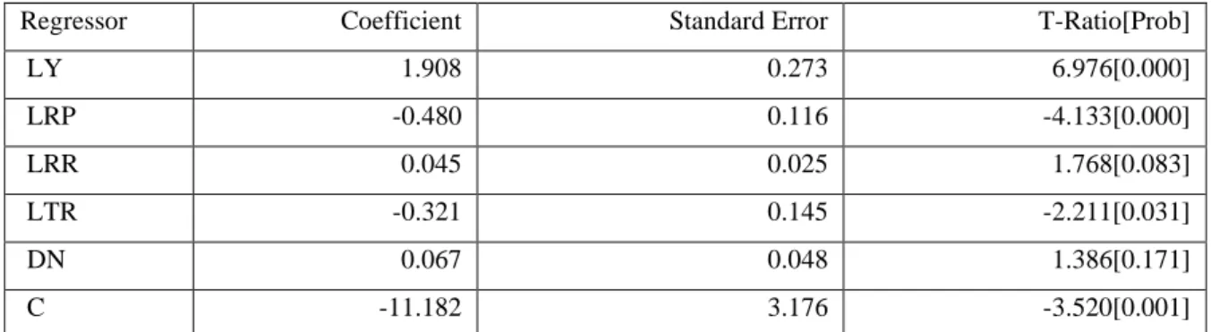
Table 4 shows the elasticity of long-run variables in the role of import demand for Bangladesh.
It is observed that actual GDP is found to have a strongly positive and statistically significant effect on import demand in the long run. This finding is found to be consistent with those already found by Hossain (2013), Lopez (2005), Aydin et al. (2004), Hussain (2004), Islam and Hassan (2004), Dutta and Ahmed (1999), Siddique (1997), Carone (1996), Nguyen and Bhuiyan (1977), Shilpi (1990) and Kabir (1988). As a result, this study just contributes to the widespread precision of the results in regarding the long association among import demand and actual GDP. But the negative and highly statistically significant coefficient of relative price designates that demand for import is adversely influenced with the rise in relative price in the
long run. This long-run negative association among relative price and import demand draws support from several studies such as Hussain (2004), Islam and Hassan (2004), Carone (1996), Kabir (1988) and Shilpi (1990).
Table 4: Projected long-run coefficients in the ARDL model
Regressor Coefficient Standard Error T-Ratio[Prob]
LY 1.908 0.273 6.976[0.000]
LRP -0.480 0.116 -4.133[0.000]
LRR 0.045 0.025 1.768[0.083]
LTR -0.321 0.145 -2.211[0.031]
DN 0.067 0.048 1.386[0.171]
C -11.182 3.176 -3.520[0.001]
ARDL method (1,0,0,0,0,0) chosen considering Schwarz Bayesian Criterion: Import demand is the dependent variable.
As expected, in the long run, real reserves have a positive association with import demand, which indicates that a rise in real reserves drives import of the Bangladesh economy. This finding also draws support from some studies, including Kabir (1988), Shilpi (1990) and Dutta and Ahmed (1999), which estimated the cumulative import demand in Bangladesh. With regards to tariff rate, it adversely affects the long-term import demand. This observation theoretically shows that, because of the imposition of tariffs, the real price of imported commodities rises and that pulls off the demand of those imported commodities in the economy. This finding goes in line with Hoque and Yusop (2010), Lopez (2005), Santos- Paulino and Thirlwall (2004), Islam and Hassan, (2004) and Kabir (1988), who found that in Bangladesh, the liberalisation of trade through the decrease of the import obligation significantly upsurges short run total import, but in the long run it does not go up to the same direction. But the finding from the ARDL approach of Hossain (2013) just contradicts this arguing that Bangladesh’s imports are actually price-inelastic, and hence, such liberalisation of trade by reducing the import duty is not fruitful. This finding is also found to be consistent with findings on some other countries such as India (Mehta & Parikh, 2005), Korea (Mah, 2000) and some other developing countries (Ju et al., 2010).
However, natural calamity has no substantial effect on Bangladesh's long-run demand for imports, indicating that the country can meet the crisis by herself without influencing the import. The result is not surprising, rather a priori could be expected, since most of
Bangladesh's import items consist of what it needs as a matter of necessity (Kabir, 1988).
Furthermore, while evidence from developing countries, as well as regions suggest that due to natural calamity, poor consumers suffer more than their richer counterparts (FAO, 2011;
D’Souza & Jolliffe, 2010; Robles et al., 2010; Subervie, 2008), but the imports of luxurious goods, which are usually demanded by richer consumer groups, are not found to have been adversely affected by natural calamity. While natural calamity seems to reduce the gap between both exporting and importing nations, governance still remains as a key factor to determine the extent of the effects of trade (Gassebner et al., 2006).
4.5 Short Run Findings
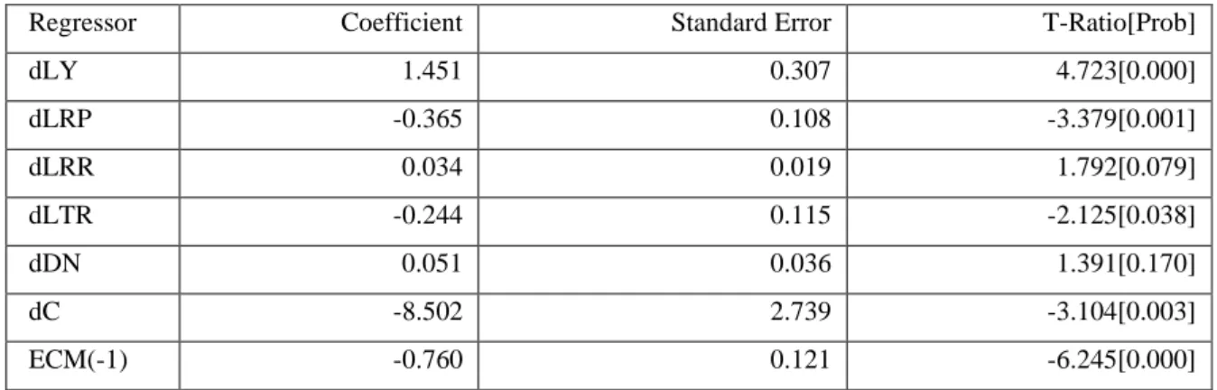
Just like the long run scenario, the real GDP has a highly positive and notable impact over short run import demand. Also, relative price and import demand are inversely associated with the short run demand. Predictably, real reserve significantly promotes import, while imposition of tariff hinders the short run import demand significantly. Since the coefficient of dummy variables of natural calamity is found to be positive but insignificant, this study cannot firmly conclude that natural calamity shrinks short run import demand. As a consequence, in both the short and long run the empirical results are already showing broad consistency. The equilibrium in the long run and disequilibrium in the short run is therefore validated by the presence of a negative and strongly statistically meaningful coefficient of Error Correction Model (ECM).
The projected coefficient of ECM is -0.76, implying that the adjustment occurs at a level of 76 percent per year towards equilibrium in the long run.
Table 5: Error rectification representations for the selected ARDL model
Regressor Coefficient Standard Error T-Ratio[Prob]
dLY 1.451 0.307 4.723[0.000]
dLRP -0.365 0.108 -3.379[0.001]
dLRR 0.034 0.019 1.792[0.079]
dLTR -0.244 0.115 -2.125[0.038]
dDN 0.051 0.036 1.391[0.170]
dC -8.502 2.739 -3.104[0.003]
ECM(-1) -0.760 0.121 -6.245[0.000]
ARDL (1,0,0,0,0,0) designated based on Schwarz Bayesian Standard.
ECM = LM - 1.9089*LY + 0.48096*LRP - 0.045547*LRR + 0.32197*LTR - 0.067306*DN + 11.1827*C
4.6 Structural Stability Test
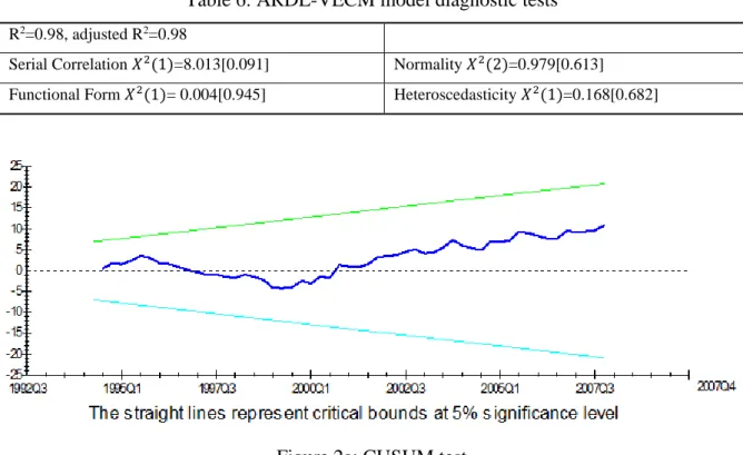
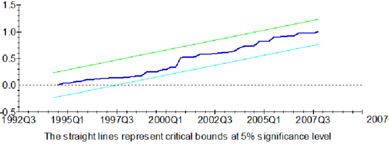
The constancy of the import demand function is critical to have productive trade policy in place. Therefore, this empirical study considers whether there has been any change in the projected import demand equation over time. The CUSUM test (Figure 2a) and CUSUM Square test (Figure 2b) conducted to check the stability of parameters shows that the variables are steady throughout the examination time. The model also passed through several other diagnostic tests. The values of R square and adjusted R square are shown as 98 and 98 percent respectively, indicating the absolute fitness of the model. Moreover, at a 5 percent level of significance, the serial correlation analysis discards the null hypothesis of no serial correlation.
The investigative tests also show that there is no functional error, abnormality, or heteroscedasticity in this model at a 10% level of significance.
Table 6: ARDL-VECM model diagnostic tests
R2=0.98, adjusted R2=0.98
Serial Correlation 𝑋2(1)=8.013[0.091] Normality 𝑋2(2)=0.979[0.613]
Functional Form 𝑋2(1)= 0.004[0.945] Heteroscedasticity 𝑋2(1)=0.168[0.682]
Figure 2a: CUSUM test
Figure 2b: CUSUM Square test
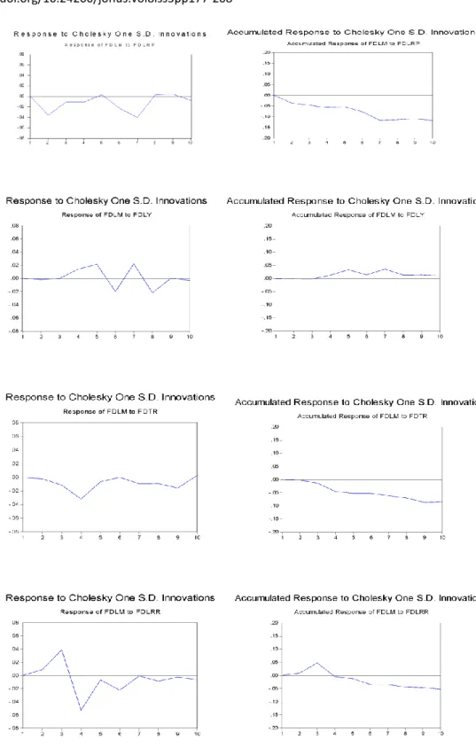
4.7 Vector Error Correction Model (VECM)
This study uses the first difference of the variables to develop impulse response functions (IRFs) in order to test the power of the ECM's outcomes. In VAR models, impulse response mechanisms examine the complex association among the factors. The impulse response function determines the time profile of stimuli impact on the expected values of variables in a complex system at a given point in time. The IRFs represent each variable's dynamic response to disruptions from other variables in the model. The receptiveness of import demand to disruptions, relative price, tariff rate, and natural calamity dummy is anticipated to be negative.
Nevertheless, it is projected that there will be a positive reaction of import demand (M) to shocks of real income (actual GDP) and reserves. In the context that a change in real GDP raises import demand, while a change in relative price reduces import demand; therefore, the impulse response may help the contention of the solitary equation method. Import demand is negatively affected by a standard deviation shock to relative price, as shown in Figure 3.
Similarly, the impact of an actual reserve shock is in line with the outcomes of a single equation study. Import demand has a positive cumulative response to the real reserve shock. The VAR result can endorse the proof of the single equation method since import demand reacts negatively to a change in tariff rate. Figure 3 shows a declining impact of one standard deviation shock to tariff rate after two (02) quarters, and the decreasing effect is highest in the fourth (04) quarter, and after that time it starts increasing.
Figure 3: Impulse Response Functions (IRFs)
Figure 3 also shows that a change in actual reserve of one standard deviation has an instant positive effect on import demand. In this case, the immediate increase in import demand lasts for two (02) quarters and continues until the fourth (04) quarter. According to the VAR analysis, the degree of reaction in import demand with various shocks of factors like tariff rate
and actual foreign exchange reserve is in line with economic instinct and the outcome of single equation analysis.
5.0 CONCLUSIONS
The purposes of this study were threefold. First, to find the influence of trade liberalisation, measured by the tariff rate, on import demand of the same at an aggregate level. Second, to gauge the determinants of Bangladesh's aggregate demand function for merchandise imports.
Third, to observe any impact of natural calamity on aggregate import demand as well as trade balance of Bangladesh. The method of cointegration and error correction was used to perform an empirical study of Bangladesh's aggregate demand function for merchandise imports. The outcome of the error correction model reveals that the variables such as import volume, relative import prices, real GDP, reserves, and tariff rates, have long-run equilibrium linkages.
Furthermore, the implementation of the error correction model was discovered to be statistically significant, indicating that the relationship is legitimate. In the estimated ECM, relative price and real foreign exchange reserve identified as significant indicators of Bangladesh's import demand function, while the real GDP and tariff rates are not found to be significant to that extent. But both the variables are found with appropriate signs and in line with the economic intuition. The estimated coefficient of error correction term in the model is 0.308, indicating that the model has a slow adjustment speed, and will experience a period of market disequilibrium before reaching long-run equilibrium. Therefore, the price and income elasticity were discovered to be statistically significant with their respective signs in the long run.
From the VECM, the accumulated impulse response, the trend of the real GDP, relative price, real reserve and tariff rate have been found consistent with their respective signs. That means the aggregate import demand increases with a standard deviation shock to real GDP, whereas a standard deviation shock to relative import price decreases the aggregate import demand. Again, a standard deviation shock to real foreign exchange reserves increases the import demand. The effect of tariffs is expressed in the commodity's import price. As tariff rates are compromised, the elasticity of price appears to grow with the increase in trade liberalisation according to the impulse reaction. Moreover, the econometric projections of Bangladesh's aggregate demand feature for imports suggest that demand for imports is primarily elucidated by real GDP, which is ultimately connected to the country's typical
economic activities. In contrast to real income, import demand seems to be sluggish to respond to changes in import rates. This study finds that the demand for imports in Bangladesh is price elastic, meaning imports can be reduced in Bangladesh when the import price rises. This indicates that increase in import prices with the imposition of tariff or non-tariff bar or depreciation of currency, i.e., devaluation may be a useful tool for limiting aggregate import demand of Bangladesh. Finally, the co-efficient of the dummy variable as a proxy for natural calamity is found with positive sign, which implies natural calamity has negative influence on the balance of trade, but the co-efficient does not show statistical significance. So, a strong policy recommendation to avoid those disturbances in the way of sustained economic development of Bangladesh can be made based on this historical finding. This study considers the historical perspective of the import demand function, which may not represent the current situation. Therefore, future study can check the validity of these historical findings by utilising updated data.
ACKNOWLEDGEMENT
This article is funded by Accounting Research Institute HICoE of Universiti Teknologi MARA and the Malaysian Ministry of Higher Education.
REFERENCES
Ahmed, N. (2001). Trade liberalization in Bangladesh: An investigation into trends.
University Press Limited.
Alam, M., Uddin, G., & Taufique, K. (2009). Import inflows of Bangladesh: The gravity model approach. International Journal of Economics and Finance, 1(1), 131-139.
Alias, M. H., Tang, T. C., & Othman, J. (2001). Aggregate import demand and expenditure components in five ASEAN countries: An empirical study. Jurnal Ekonomi Malaysia, 35(2001), 37-60.
Ang, J. B. (2009). Financial development and the FDI-growth nexus: The Malaysian experience. Applied Economics, 41(13), 1595-1601.
Ang, J. B., & McKibbin, W. J. (2005). Financial liberalization, financial sector development and growth: Evidence from Malaysia. (Centre for Applied Macroeconomic Analysis Working Paper 5). Australian National University.
Arize, A. C., & Malindretos, J. (2012). Foreign exchange reserves in Asia and its impact on import demand. International Journal of Economics and Finance, 4(3), 21-32.
Arize, A. C., & Osang, T. (2007). Foreign exchange reserves and import demand: Evidence from Latin America. World Economy, 30(9), 1477-1489.
Arize, A. C., Malindretos, J., & Grivoyannis, E. C. (2004). Foreign exchange reserves and import demand in a developing economy: The case of Pakistan. International Economic Journal, 18(2), 259-274.
Aydin, M. F., Ciplak, U., & Yucel E. M. (2004). Export supply and import demand models for the Turkish economy. (Research Development Working Paper 04/09). The Central Bank of the Republic of Turkey.
Aziz, M. N. (2013). Modelling import demand function for a developing country: An empirical approach. Asian-African Journal of Economics and Econometrics, 13(1), 1-15.
Babatunde, M. A., & Egwaikhide, F. O. (2010). Explaining Nigeria's import demand behaviour: A bound testing approach. International Journal of Development Issues, 9(2), 167-187.
Bhuyan, A. R., & Rashid, M. A. (1993). Trade regimes and industrial growth: A case study of Bangladesh. Bureau of Economic Research, University of Dhaka.
Brandt, L., Van Biesebroeck, J., Wang, L., & Zhang, Y. (2017). WTO accession and performance of Chinese manufacturing firms. American Economic Review, 107(9), 2784-2820.
Carneiro, F. G., & Arbache, J. S. (2003). The impacts of trade on the Brazilian labor market:
A CGE model approach. World Development, 31(9), 1581-1595.
Carone, G. (1996). Modeling the US demand for imports through cointegration and error correction. Journal of Policy Modeling, 18(1), 1-48.
Chimobi, O. P., & Ogbonna, B. C. (2008). Estimating aggregate import-demand function in Nigeria: A co-integration approach. Journal of Research in National Development, 6(1), 234-256.
D’Souza, A., & Jolliffe, D. (2010). Rising food prices and coping strategies: Household-level evidence from Afghanistan. (World Bank Policy Research Working Paper 5466). The World Bank.
De Mel, S., McKenzie, D., & Woodruff, C. (2012). Enterprise recovery following natural disasters. The Economic Journal, 122(559), 64-91.
Dutta, D., & Ahmed, N. (2004). An aggregate import demand function for India: A cointegration analysis. Applied Economics Letters, 11(10), 607-613.
Dutta, D., & Ahmed, N. (1999). An aggregate import demand function for Bangladesh: A cointegration approach. Applied Economics, 31(4), 465-472.
Emran, M. S., & Shilpi, F. (2010). Estimating an import demand function in developing countries: A structural econometric approach with applications to India and Sri Lanka. Review of International Economics, 18(2), 307-319.
Emran, M. S., & Shilpi, F. (2001). Foreign Trade regimes and import demand function:
Evidence from Sri Lanka. SSRN.
Engle, R. F., & Granger, C. W. (1987). Co-integration and error correction: Representation, estimation, and testing. Econometrica, 55(2), 251-276.
Ernst, C. (2005). Trade liberalization, export orientation and employment in Argentina, Brazil and Mexico. ILO, Employment Analysis Unit.
FAO. (2011). The state of food insecurity in the World - How does international price volatility affect domestic economies and food security? Food and Agriculture Organization of the United Nations.
Fatukasi, B., & Awomuse, B. O. (2011). Determinants of import in Nigeria: Application of error correction model. Centrepoint Journal, Humanities Edition, 14(1), 52-72.
Fosu, O. E., & Magnus, F. J. (2006). Bounding testing approach to cointegration: An examination of foreign direct investment trade and growth relationships. American Journal of Applied Sciences, 3(11), 2079-2085.