No5JalanGelangll/6A, Dr fi^ry&aierak. Malaysia - UTPedia

Title of thesis

STATUS OF THESIS

Numerical Modelling and Simulation of Bone Drilling to Minimize Bone Necrosis by Controlling Heat Generations

MUNAIBAH BINTIMOHD MOKHTAR

hereby allow my thesis to be placed at the Information Resource Center (IRC) of Universiti Teknologi PETRONAS (UTP) with the following conditions:

1. The thesis becomes the property of UTP

2. The IRC of UTP may make copies of the thesis for academic purposes only.

3. This thesis is classified as

Confidential

/ Non-confidential

If this thesis is confidential, please state the reason:

The contents of the thesis will remain confidential for years.

Remarks on disclosure:

Endorsed by

iu&^

Signature of Author Signatd^ofisirpervisor

^ °SeniorLecturer*' Department

Permanent address: Narfle'<?f%ffl^|^v

No5JalanGelangll/6A, Dr fi^ry&aierak. Malaysia

Seksyen 11 40100, Shah Alam Selangor.

Date : 29 July2013 Date • 29 July 2013

UNIVERSITI TEKNOLOGI PETRONAS

NUMERICAL MODELLING AND SIMULATION OF BONE DRILLING TO MINIMIZE BONE NECROSIS BY CONTROLLING HEAT

GENERATIONS

by

MUNAIBAH BINTIMOHD MOKHTAR

The undersigned certify that they have read, and recommend to the Postgraduate 5Studies Programme for acceptance this thesis for the fulfillment of the requirements for the degree of Master of Science in Mechanical Engineering.

Signature:

Main Supervisor:

Signature:

Co-Supervisor:

Signature:

Head of Department:

Date:

Dr Hasari

IFawad fcturer

al Engineering Department Teknologi PETRONAS Bandar Sen iskandar

3-pso Tronoh. PeraK, Malaysia

Dr Anis Suhaila binti Shuib

wu»auHM*aHu»

Ucfvnr

Cham. Eng-Department

Dr Ir Masri Bin Baharom

29 July 2013

Ir. Dr. Masri Baharom

Head of Department/Associate Professor Department of Mechanical Engineering Universiti Teknologi PETRONAS Bandar Seri Iskandar, 31750 Tronoh, PeraK uarui Ridzuan, Malaysia

NUMERICAL MODELLING AND SIMULATION OF BONE DRILLING TO MINIMIZE BONE NECROSIS BY CONTROLLING HEAT GENERATIONS

by

MUNAIBAH BINTIMOHD MOKHTAR

A Thesis

Submitted to the Postgraduate Studies Programme as a Requirement for the Degree of

MASTER OF SCIENCE

DEPARTMENT OF MECHANICAL ENGINEERING

UNIVERSITI TEKNOLOGI PETRONAS

BANDAR SERI ISKANDAR

PERAK

JULY 2013

DECLARATION OF THESIS

Title of thesis Numerical Modelling and Simulation of Bone Drilling to Minimize Bone Necrosis by Controlling Heat Generations

I MUNAIBAH BINTI MOHD MOKHTAR

hereby declare that the thesis is based on my original work except for quotations and citations which have been duly acknowledged. I also declare that it has not been previously or concurrently submitted for any other degree at UTP or other institutions.

^L^

Signature of Author

Permanent address:

No 5 Jalan Gelang 11/6A, Seksyen 11 40100, Shah Alam Selangor.

Date : 29 July 2013

Witnessed by

n Fawad

cluier .

„w.«..3HIKptt»flns Department Universiti Teknologi PETRONAS

Namef^^lrinfplerS. Malaysia

Dr Hasan Fawad

Date: 29 July 2013

DEDICATION

To my mom, dad, husband and brother for their love and supports in this journey.

ACKNOWLEDGEMENT

* vAllah the Almighty, for without His consent it would

FirstofalUwouldliketothankAllahtheAlrmgJ, he strength

be possible to achieve what has been done mthis ^ « this work

and perseverance to keep going without losmg hope. May Allah

count it as agood deed and make it useful to others.

« Ahv University Technology Petronas, through a This research was supported by University

, t, TITP Graduate assistantship fund to the first author and

St^Ci *.« «o the second. The secon, author , - ^wi.UTP-CoECent.eroH^entS^-^insKe^cMCISm).

it in its best condition.

Tta experiment was success** done with the help of lab technician Mr Hazif

The expenment ^^ b^ Yusoff md Nmll

bin Safian. Zulkamam Jahdi BNordrn, W ^ ^

AizatBtNgah from the Centre of Graduate stud.es (COS) also

££1- ht debt and than*, with their guidance and Kndness „n*ng thts

researchpossible.

ABSTRACT

Bone drilling method is one of the medical approaches to handle fracture in trauma injury. It involves the insertion of a screw and/or a plate for temporary support. However, drilling generates heat thus causing thermal necrosis. The temperature which reach above thermal necrosis threshold during drilling causes two problems; the bone tissue losses its regeneration ability and loosening of the surgical fixation over time. This project aims to develop appropriate numerical heat transfer model adaptation of the heat source approach for bone drilling with the purpose of minimizing thermal necrosis. Method of investigations used were numerical modeling and simulation using ANSYS parametric design language (apdl). The relationship of drill speed, feed rate, point angle, helix angle and drill bit diameter were investigated using the heat source model. Prediction of the temperature distribution and a parametric study was conducted. The analysis have been validated by using dry bovine bone. Analytical and experimental results of this study suggested that the feed rate, drill bit diameter and point angle have 11.63%, 73.44% and 25.60% influential on heat generation respectively.

Prediction of temperature distribution shows a decrease of 35.47% and 17.43%

in temperature with the use of 0.42 mm/s feed rate as compared to 2.2 mm/s and 40° point angle as compared to 118° respectively, while 70.34% increased with the use of 4.5 mm drill bit diameter as compared to 1.5 mm. Thus, the appropriate drilling condition is recommended by using drill bit diameter lower than 3.5 mm, feed rate more than 1.2 mm/s and point angle of 118°.

ABSTRAK

Kaedah penggerudian tulang digunakan dalam bidang perubatan untuk menyambung semula tulang yang patah semasa kecederaan trauma, ia dibuat dengan menggerudi plat atau skru ke dalam tulang tersebut untuk memperolehi sokongan yang sementara. Akan tetapi proses penggerudian ini akan menghasilkan haba nikrosis, jika haba tersebut melebihi had kecederaan tulang, ia akan mengakibatkan masalah kehilangan keupayaan untuk baik sepenuhnya.

Fokus penyelidikan ini adalah untuk meminimakan kecederaan tulang dengan memperolehi parameter sesuai untuk pengerudian tulang tersebut. Kaedah yang digunakan adalah pembinaan model numerasi dan simulasi ANSYS menggunakan parametric design language (apdl). hubungkait antara kelajuan gerudi, kelajuan putaran, sudut titit, sudut heliks dan bit diameter gerudi telah diberi tumpuan kajian dengan menggunakan model sumber haba (Heat Source Model). Jangkaan tentang taburan suhu dan kajian tentang parameter tersebut telah dijalankan. Kajian telah dijalankan dengan menggunakan tulang bovin yang kering. Hasil kajian secara eksperimen dan analitikal menunjukkan bahawa kadar putaran, bit diameter gerudi dan sudut titik mempengaruhi sebanyak 11.63%,

73.44% dan 25.60% ke atas penghasilan haba masing-masing. Jangkaan tentang

pengaruh haba pula menunjukkan penurunan suhu sebanyak 35.47% dan 17.43%

apabila menggunakan 0.42 mm/s kadar putaran berbanding dengan kadar putaran

2.2 mm/s dan memilih sudut titik 40° berbanding dengan sudut 118° masing-

masing. Maka keadaan penggerudian yang menasabah adalah dengan

menggunakan bit diameter gerudi yang kurang daripada 3.5 mm, kadar putaran

yang lebih daripada 1.2 mm/s dan sudut titik 118°.

In compliance with the terms of the Copyright Act 1987 and the IP Policy of the university, the copyright of this thesis has been reassigned by the author to the legal entity of the university,

Institute of TechnologyPETRONAS Sdn Bhd.

Due acknowledgement shall always be made of the use of any material contained in, or derived from, this thesis.

© Munaibah Mohd Mokhtar, 2013 Institute of Technology PETRONAS Sdn Bhd All rights reserved.

TABLE OF CONTENTS

STATUS OF THESIS i

DECLARATION OF THESIS iv

ACKNOWLEDGEMENT vi

ABSTRACT vii

ABSTRAK viii

LIST OF TABLES xii

LIST OF FIGURES xiii

LIST OF EQUATION xv

CHAPTER 1 INTRODUCTION 16

1.1 Overview 16

1.2 Background of Study 16

1.3 Case Study 17

1.4 Problem Statement 18

1.5 Objective of the Research 19

1.6 Scope of Research Project 20

1.7 Layout of Thesis 20

1.8 Summary 22

CHAPTER 2 23

2.1 Overview 23

2.2 Thermal Necrosis 23

2.3 Parametric Experiments and itsConflicts 24

2.4 Importance of Finite element modelling 25

2.5 Numerical Modelling 26

2.5.1 Heat generation 26

2.5.2 Heat Source Model 31

2.6 Finite Element Theory 32

2.6.1 Modeling Concepts 32

2.6.2 Finite Element Simulation 35

2.6.3 Model construction 36

2.7 Experimental Approach 42

2.7.1 Properties of bone 42

2.7.2 Temperature measurement 45

2.8 Summary 46

CHAPTER 3 47

3.1 Overview 47

3.2 Numerical Modeling and Analysis 49

3.3 Modeling 50

3.3.1 Model Geometry 52

3.3.2 Material Properties 55

3.3.3 Meshing 55

3.3.4 Time Step 57

3.4 Experimental Validations 57

3.4.1 Experimental apparatus 58

3.4.2 Sample Preparations 58

3.4.3 Experimental Procedure 58

3.5 Summary 60

CHAPTER 4 61

4.1 Overview 61

4.2 Relationship between parameters and heat generation 62

4.3 Finite Element Modeling 66

4.4 Validation 66

4.5 Parametric Analysis 70

4.5.1 Effect of feed rate 71

4.4.2 Effect of point angle 73

4.5.2 Effect of drill diameter 75

4.5.3 Effect of drill motion at point A 77

4.6 Summary 78

CHAPTER 5 79

5.1 Conclusions 79

5.2 Recommendation for Future Work 80

REFERENCES 81

LIST OF TABLES

Table 2.1 Material properties ofbone used inFEM 43

Table 2.2 Bone sample preparations 43

Table 3.1 Surgical geometries 50

Table 3.2 Model dimension in FE 53

Table 3.3 Mechanical characteristic of the bone used in FEM analysis 55

Table 3.4 Initial meshing procedure 56

Table 4.1 Parameters tested in MATLAB 63

Table 4.2 FE simulation ^

Table 4.3 FE(1) and experimental approach 66

Table 4.4 FE(II) and literature reference approach 68

Table 4.5 Parametric case study 71

LIST OF FIGURES

Figure 1.1 (a) Lateral radiograph of femoral fracture in a 7-month-old dog. (b) the fracture following reduction and fixation using a bone plate and screws, (c)

Radiograph after 5 months [1] 16

Figure 1.2 Sequential development of biochemical and morphologic changes in cell

injury [2] 17

Figure 1.3 Radiographic appearance of thermal necrosis [7] 18 Figure 2.1 Material removal by orthogonal cutting [8] and [30] 28

Figure 2.2 Drill bit geometry [30] 31

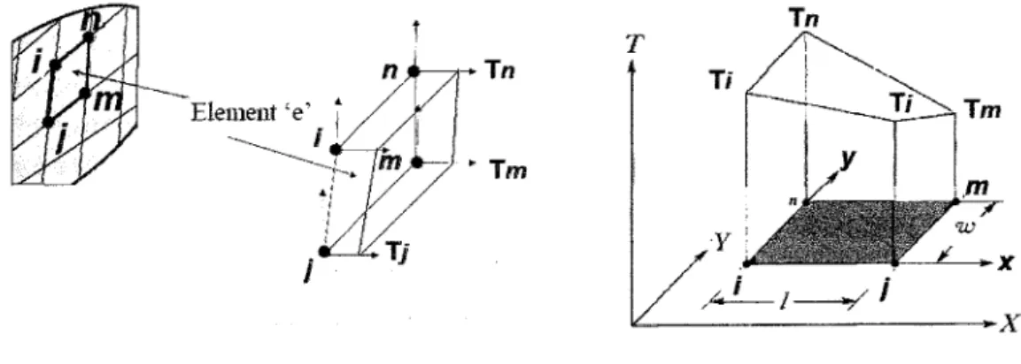
Figure 2.3Using two-dimensional rectangular element to describe temperature distribution, x,y is local coordinate and X,Y is global coordinate system.33

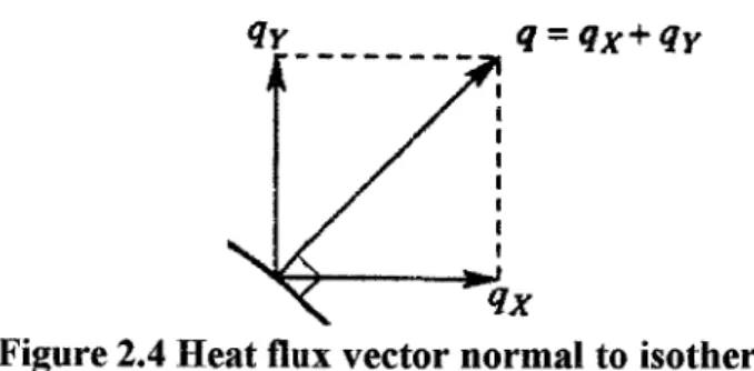
Figure 2.4 Heat flux vector normal to isotherm 35

Figure 2.5 Geometrical model of the disc simulated of bone 37 Figure 2.6 Assigning material properties ie density from CT scan of bone to FE bone

model [60] 40

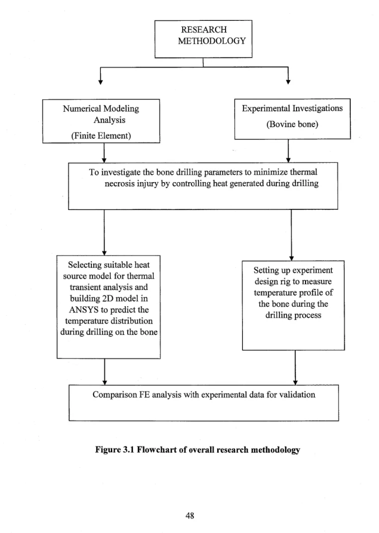
Figure 3.1 Flowchart of overall research methodology 48

Figure 3.2 Flowchart of numerical analysis 50

Figure 3.3 Flowchart of optimization procedure 51

Figure 3.4 Flow of loop command used to simulate drilling process using heat flux

input data 54

Figure 3.5 Session editor of ANSYS apdl for one load step 55 Figure 3.6 Effect of integrationtime step on maximum nodal temperature 57 Figure 3.7 (a) overall view ,(b)The thermocouple and drill bit position, (c) Approximation of 3mm distance from the drill bit and the thermocouple, (d) overview of how thermocouple data logger were connected,(e) the height level of thermal imaging camera were taken, (f) the bone condition

after drilling 60

Figure 4.1 Relationship between parameter stated in table 4.1 with heat generation. 63 Figure 4.2 Relationship between influential parameters as a function of drilling speed

65

Figure 4.3 Graph of FE(I) and experimental method 67

Figure 4.4 Thermal imaging showing maximum temperarure of 50.3°C for drilling

speed of 16,000 rpm 68

Figure 4.5 Graph of FE(U) and Literature reference 69

Figure 4.6 Maximum nodal temperature for Case 1

71

Figure 4.7 Representing case 1with variation ofdrilling speed, rpm 71 Figure 4.8 Representing case 1with variation depth ofcut, mm 72

Figure 4.9 Maximum nodal temperature for case 4

73

Figure 4.10 representing case 4with variation of drilling speed, rpm 73

Figure 4.11 representing case 4with variation depth of cut, mm

IA

Figure 4.12 Maximum nodal temperature for case 3

75

Figure 4.13 representing case 3with variation ofdrilling speed, rpm 75 Figure 4.14 representing case 3with variation depth of cut, mm 76

Figure 4.15 Representing case 6

77

Figure 4.16 Representing case 7

77

Figure 4.17 Representing case 8

78

LIST OF EQUATIONS

(2.1) t.43 = t = Ot = tfinalR(Tt)43-Ttdt 24

(2.2) RTt = 0.5 if Tt > 43°C0.25 otherwise 24

(2.3) dQdt = Fsvs 27

(2.4) vs = Vcoscf) 27

(2.5) 24 = 90°+ /3-a 27

(2.6) tan(a) = 2rDta.nO - tansin - lrfo2rsinpcosp sinp 28

(2.7) v = 2nrN60 28

(2.8) a = tl216C2sin4(0)[tana + cot(0)] 28

(2.9) yAB - I74(va)sin20tana + cot032 28

(2.10) xs oc 80k450.06 29

(2.11) xs = BOyABO.06 29

(2.12) As = tl(D - do)cos90° - psin0 29

(2.13) tl = /2iV60sinp 29

(2.14) dQwdt = ndQdt = nAsxsvs 29

(2.15) 7/(0 = bl + b2x + b3y + bAy 33

(2.16) T = Tn at x = 0 and y = w 33

(2.17) 64 = llw(Ti - Tj + Tm- Tn) 33

(2.18) 7/(e) =Si SjSmSnTiTjTmTn 34

(2.19) Sn = ywl - xl 34

(2.20) ifj(e) = SiSjSmSnipijxjjmtpn 34

(2.21) q"Y = -kAdTdY 34

(2.22) kxd2TdX2 + kyd2TdY2 + q' 35

(2.23) -kdTdXxO = q"o 35

1.1 Overview

CHAPTER 1 INTRODUCTION

This chapter introduces the broad overview of this research topic. The chapter describes the background of this study, case study, general description of the topic which based on actual problem that have been faced. Apart from that, the problem statement is presented to describe what are the patient and doctor problems regarding bone fracture injury and this will strengthen the reason of why this study is important to be undertaken. This chapter includes the established objectives and scope of this research. In the last section of this chapter, the layout of this thesis was described.

1.2 Background of Study

Figure 1.1 (a) Lateral radiograph of femoral fracture in a7-month-old dog. (b)

the fracture following reduction and fixation using abone plate and screws.

(c) radiograph after 5 months [1]

Figure 1.1 above shows a fracture occur in dog aged 7 months. The medical

approached used were to insert screw and plate as atemporary support. Inserting the

plate and screw into the bone required drilling, which cause thermal necrosis under

certain circumstances. This project focuses on minimizing thermal necrosis by obtaining process parameter during the bone drilling procedure. The problem regarding thermal necrosis occurs are; (1) possibility of reoperation, (2) the bone lost its regeneration ability and (3) loosening of implants after surgery. Prediction of the temperature distribution during drilling may help in determining the recommended parameters to be used in order to minimize the thermal necrosis.

1.3 Case Study

Reversible ' liremsbk?

ee!< m|ury [ eei; w.ujy

> Biochemical I alterations

Uitfasfrxtura' I tgnt

claiges rwcroscoptc changes

Tiorphoi^gtc ' r.hances

DJ3AT-0*. OF INJUR"-"

Figure 1.2 Sequential development of biochemical and morphological changes in cell injury [2]

Figure 1.2 shows morphology of cell injury, irreversible cell injury occurs after a certain period of time when the stress or thermal effect had been applied for a longer duration. Cell becomes nonfunctional after biochemical alteration thus resulting death of cell. Thermal injury induced during bone drilling procedure often caused irreversible damage, where the bone cell loss its regeneration ability and properties.

A study was conducted by Neander et al, [3] to determine if bone loss is reversible after necrosis, the measurements were repeated 3 and 6 months later, which failed to note any restoration of bone mineral. Ahl et al, [4] and Finsen [5] also failed to note reversibility of bone density after an ankle fracture.

Failures of implant fixation were also due to thermal injury. The heat generated during bone drilling cause transient temperature between the bone and the drill bit.

Berning et at [6] investigate acase of proximal tibia due to thermal necrosis of pin tracker placement. Matthews et at [7] measure temperature and time during insertion of different type skeletal immobilization pin in human cortical bone, they found that thermal necrosis can be presented in radiographic as ring around the drilling hole as

shown in Figure 1. 3 below;

Figure 1.3 Radiographic appearance of thermal necrosis [7]

1.4 Problem Statement

The drilling process generates heat due to the (1) friction of the drill bit to bone and (2) as aresult from material removal. Temperature that reach above thermal necrosis threshold during drilling cause two problems. First, the bone tissue lost its regeneration ability. Second, loosening of the surgical fixation over time. In our current project, we (1) identify the heat source model and obtaining the heat flux, (2) predict the temperature distribution during drilling using heat flux data, (3) validating the temperature distribution by comparing experiment and literature review reference and (4) carry out parametric analysis. Our aim in this project is to determine the

parametric estimation that could minimize thermal necrosis.

In this study, we develop numerical heat transfer model for bone drilling, and validating the model by comparing it with data from literature review and experimental to determine suitable process parameter that could minimize thermal

necrosis.

1.5 Objective of the Research

Develop numerical heat transfer model to predict drilling temperatures as a function of process parameters and the validation of model by building a test rig to perform the drilling experiments. To accomplish this, following objectives have been carried out

as follows:

1. To develop numerical heat transfer model for bone drilling using heat source 2. To develop a Finite Element model in ANSYS Parametric Design Language

(apdl) and to set up a laboratory scale test rig to measure temperature during drilling for bovine bone as a validation for the modelling.

3. To carry out parametric analysis of minimization thermal necrosis for bone drilling method.

Based on the above objectives, there are a few questions which this research seeks

to answer.

1. If there are some differences in the heat source modeling, what are the trends of calculated heat flux and what are their relationships?

2. If there are some differences in the 2-dimensional modeling, what are the trends of temperature distribution prediction and what are their relationships?

3. What are the reasons for producing dissimilarity of predicted temperature distribution data compare to the experimental and literature review data?

4. Is there any adjustments which can be done to produce identical temperature distribution data and what are their correction factors after the adjustment?

These are the initial questions which enabled the study to create objectives for this research work. The questions seek to show the direction to efficiently run this research and facilitate research investigation. In the following section, the scope ofthe research project related to the above established objectives is discussed.

1.6 Scope of Research Project

Heat modeling is the prediction of heat transfer using mathematical equations. Heat transfer equation such conduction and convection were paired with thermo-mechanics of the drilling operation. This research covers the heat modeling from Davison and James. Davison and James [8] developed thermo-mechanical equation of the machining theory to predict heat transfer during drilling The heat models are further

discussed in the next chapter

Heat source modeling are used to calculate the dependency of the heat generation

upon the (1) drill speed, (2) drill bit diameter, (3) feed rate, (4) helix angle, and (5) point angle. Heat generation were controlled by varying those parameters. Thus these

parameters were further discussed in the chapter 2and 3.

The FE model are build using ANSYS apdl transient thermal analysis. The model will be built in 2-dimensional and the material properties of the bone will follow all literature review references that will be further discussed in the next chapter. The FE model stability is proven by conducting experimental validation.

1.7 Layout of Thesis

The thesis is comprised of five (5) chapters as follows;

Chapter 1Introduction; this introductory chapter describes the background of this research work, problem statement, objectives and scope of the research project. This chapter also answers the reasons of conducting this research and the significance

thereof.

Chapter 2Literature Review; this chapter reviews the theories and research done

in the past which is related to this research work. The context and basic terms used in

this thesis and examples are explained. This chapter demonstrates an idea about the importance of this study by showing the current knowledge and understanding which include the findings from the previous bone drilling studies that have been accomplished.

Chapter3 Methodology; this chapter explains the process of this research work by

showing the overall research work and elaborates on the methods of research analyses. Appropriate methodology flow and approach would be able to make the objective of this research measurable. The first objective of this research is to develop numerical heat transfer model for bone drilling. Heat generated at the bone during drilling via shearing process, which is similar to the machining, thus machining equation is used to develop heat model. The selected equation will be solved using

Finite Element method, ANSYS software is selected to solve this numerical implementation. MATLAB would be used to identify which parameters in these equations are important. After identifying the parameters, those parameters will be

used in ANSYS for the heat model simulation.

This chapter also includes the bone modeling approach. In this project the model were built manually using tools in ANSYS. Modeling is effective as it simplifies the current problem, but the value inserted need to be as close as possible resembling the

nature of the material. The material model values inserted follows literature review

reference mentioned in chapter 2.

Chapter 4 Results and Discussion; this chapter answers the hypothesis of this research project. It discusses the analysis of the accomplished results, findings and the implications of these findings. This will provide the estimation of the bone drilling process in medical aspects.

Chapter 5 Conclusion and Recommendations; in this chapter, conclusions are made based on the results of this research work to answer the established objectives.

This chapter summarizes the accomplished findings. This is the final chapter of this thesis. The chapter presents some recommendations in order to enhance and develop this study in the future. It may help to guide future research works or other related works in order to achieve more accurate and reliable results. The recommendations

provide future direction in bone modeling simulation for the improvement of medical purpose . This will aid in reaching an optimum design leading to the safer surgery.

This chapter is extremely valuable to other studies in order to achieve greater levels of

the research.

1.8 Summary

This chapter discusses the importance of the project in aiding medical fields with parameter data. The background of the studies provides grandness information needed

for this research. The problem statement, objectives, scopes assists for the solid frameworks. Lastly, the layout of the thesis shows an overview of how this research

has been carried out.

CHAPTER 2 LITERATURE REVIEW

2.1 Overview

Critical literature reviews of the subjects were explained in details, this chapter is divided into three phases;

i. Numerical modeling

ii. Finite element simulation

iii. Experimental approach for bone drilling validation

The first phase discusses about the term of thermal necrosis. Evaluation of the numerical modeling method to predict the heat generations using machining equation

were discussed in details.

The second phase explains in depth about finite element modeling, hence the works of finite element modeling regarding bone drilling method were discussed.

The third phase explicated the experimental approach done to predict the temperature distribution of bone drilling. The reasoning of the method was used as importance guidance for conducting the experimental validation part.

2.2 Thermal Necrosis

Thermal necrosis or the death of bone cell caused irreversible damage, which may lead to problems such as infections and the reduction of mechanical strength of the bone [9]. Hence it is important to understand the extent of necrosis, Eriksson and Albrektsson [10] found that it depends on the duration and temperature exposure.

Lundskog [11] states that if bone is exposed longer than 30 s at 50°C cellular necrosis will occur. Mortiz and Henrique [12-13] found that when epithelial cells are exposed to a temperature of 70°C they will be immediately damaged. At the exposure of 55°C for 30 s, the result will be the same and at a temperature of 45°C harmful effects will

occur after 5 h. Generally, the literature shows that if the temperature rises above 55°C for aperiod of longer than one-half aminute, serious damage will occur to the bone. Concept of thermal exposure is also define by Sapareto and Deway [14] as ;

t43 = ft=tfinal R(T(t))43-rW df (2.1)

R{Ht))- I 0.25 otherwise,

where Uis exposure time at 43°C ,tf,„a. is the period of exposure, Ris acoefficient

of exposure, and T(t) is the temperature at the certain point or location. Assumption of

necrosis threshold of 120 equiv. min at 43°C were debated. However, it is commonly

accepted that exposure time value is depending at different tissue type under different

clinical condition. This project follows Eriksson et al. [15] suggested thermal necrosis threshold, which are initiated when the temperature exceed 47 °C for 60s.

Complying with equation (2.1) and (2.2) t43 is equal to 16 min.

2.3 Parametric Experiments and its Conflicts

Some researchers found out that by increasing the drilling speed itwould significantly increases the temperature generated at the bone [16] and [17] but those result were conflicted with [18], [19] and [20] which stated that drill bit with higher drill speed can reduce the bone temperature rise.The methods of direct experimental approach are expensive and time consuming. There are various parameters influencing temperature distribution during bone drilling. However, those parameters have complex relationship; the relationship between the drill-bit geometry, chip stream, drilling conditions, and bone characteristics possess a great challenge to determine which parameter is favourable. Thus making the optimization of parameters to minimize the

thermal effects in experimentation alone is impractical. Due to that, recently the finite element simulation is widely used to investigate the mechanism ofcutting process. It is also an effective and efficient way to model the process and gain better

understanding of the operations.

2.4 Importance of Finite element modelling

Numbers of researchers have developed analytical models. Loewen and Shaw [21]

proposed a prediction of heat partition based on Jaeger's analysis. The model was improved by Agapiou and DeVries [22], who tailoring it to be able to predict thermal phenomena in drilling by developing analytical model for twist drill temperature and used the model for comparison of experimental and analytical. Kalidas et al. [23]

investigated influences of drill temperature on hole quality under dry and wet drilling conditions. Later on Agapiou and Stephenson [24] made a subsequent improvement.

Other than that, Watanabe et al. [25] also used Loewen and Shaw model to predictthe heat flows into the workpiece and the drill. As mentions, Loewen and Shaw model were widely used, however it is too simplified. For example the model assume that the temperature induced in the workpiece on the shear plane is similar or equivalent in some respects to the temperature beneath a frictional slider that dissipates uniform heat flux as it moves with constant speed over the surface of a semi-infinite body. As a result, the classical model can be inaccurate for cutting scenarios that involve large shear angles or slow cutting speeds, which occur commonly in drilling.

The method of direct experimental approach to studies the drilling process and its parameter are expensive and time consuming. Due to that, recently the finite element simulation is widely used to investigate the mechanism of cutting process. It is also an effective and efficient way to model the process and gain better understanding of the operations. Yang and Sun [26] investigated drilling process; a coupled thermo- mechanical finite element model of drilling is developed. Several key technologies, such as material constitutive model, material failure law, contact and friction law, have been implemented to improve the accuracy of finite element simulation. And by comparing the predicted cutting forces with the measured forces shows the finite element model is reasonable. These results confirm the capability of finite element simulation in predicting drilling process and selecting optimal tool and cutting parameters, due to this, long and lengthy experimentation train and error could be

minimize.

Many physical phenomena in engineering and science can be described in terms of partial deferential equations (PDE). In general, solving these equations by classical

analytical methods for arbitrary shapes is almost impossible. The finite element method (FEM) is a numerical approach by which these PDE can be solved approximately. The FEM is a function/basis-based approach to solve PDE. FE is

widely used in diverse fields to solve static and dynamic problems, in this case we are solving complex geometry of drill and how its influence heat generations. In additions, there are lots studies and investigations on drilling, turning, milling and grinding using finite element simulations. Like to those in bone drilling, the thermal

effects in metal drilling are caused by heat generation resulting from material shearing which undergo plastic deformations and frictions. For example Davison and James [27]used machining theory developed by Tay et. Al. [28] to predict the heat transfer

during drilling and by coupling it with FE.

2.5 Numerical Modelling

Numerical modeling basic concept involves solving a physical problem by simplification of the reality. Approach to theoretical method consist of four steps;

constructing the mathematical model closely resemble the physical problem with assumption, development of the approximation of mathematical model, obtaining solution by implementing the numerical model and interpretation of those data.

2.5.1 Heat generation

The heat generated during drilling of bone comes from; firstly, the drilling process.

Shear occurs at the surface layer ofa material by a drill bit that breaks intermolecular bonds, thus releasing energy. Secondly, the friction from the non-cutting surfaces of a twist drill, such as the flank, flutes and shaft are another source ofheat. The heat

generated is partially dissipated by the presence of blood and tissue fluid, and part of

the heat being carried away by the chips formed. But then again, bone is a poor

conductor of heat and the temperature rise canbe significant.

Heat generated from the product of shearing. As the drill bit touch the bone,

shearing of the surface layer of the bone occur. The shearing process would break the

intermolecular bonds of the bone. Intermolecular bond is the forces of attraction

which hold an individual molecule together. Breaking the bond would release energy, which is the heat generated during the process. Besides shearing, friction also influences the temperature during drilling. Frictions are the force resisting the relative motion of solid surfaces. Frictions occur from the non-cutting surfaces of a drill, such as the flank, flutes and shaft are another source of heat. Energy used to remove a material is converted into heat [29], thus heat generated by the amount of work is;

do „

—t = Fsvs

^(2.3)

where Q is the heat generated, t is time, Fs is the shearing force in the shear plane, vs is the shear velocity, and where the shear force and shear velocity are at the same angle (p. Figure 2.1 below shows the concept of material removal by orthogonal cutting

(a) _tool

shear %'eiocity, vs

chip velocity, vc

11 TnTiiiinT"""'""?1 -4" cuttingvelocity, v

wortc piece

(b) Rake

face

bone chip

Tool

(c)

Krtke

work piece

Figure 2.1 Material removal by orthogonal cutting [8] and [30]

y Rolif!

1 Angle'

Davison and James [8] mathematical model substitution in details; shear velocity is calculated by;

vs = — i_{cos cj>} (2.4)

angle (p is calculated using Ernst-Merchant relationship for bone cutting [31] by;

2<f> = 90o + p-a _(2.5)

where a is define as the rake angle ofthe cutting tool and the friction angle, 0has the value of 0.644 [31]. changes in the rake angle along the cutting lips of a drill is express by Bhattacharyya and Ham [32] and is as follows,

r ^ (2r/n)tan(g)-tan[sin-1(^/2rsinp)]cosp

tan(a) = — &*>

where Dis the drill diameter, do is chisel edge diameter, 6 is the helix angle, and/? is

the half-angle at the point (fig 2.1). The average rake angle over the length of the cutting edge was calculated by numerically integrating Eq. (2.6) over the drill radius and dividing the result by the radius. The velocity valso changes along the cutting

edges,

2nrN /•-, ^

V = <A')

60

where N is the rotational speed, in rpm. In this analysis, the average cutting velocity over the radius of the drill was used to calculate, vs Tay et &1 pgj formuia were

used to calculate the constant a,

t2L_i_ (2.8)

a —16C2sin4(tf>)[tan(a)+cot(0)]

where his the undeformed chip thickness, which in this case is the depth of cut per revolution, and C is a material constant value of6 [28]. Expression for the shear rate in the primary deformation zone, which occurs in the shear plane line AB was

calculated from:

YAB 4(Va)sin2(0)[tan(a) +cot(0)]3/z

(2.9)

With (p known from Eq. (2.5) and a known from Eq. (2.8), values of

Yab were calculated for a known rake angle, a.

Ultimate shear stress on shear rate for bone, Carter and Hayes [33] found that the

compressive strength of cortical bone is proportional to the strain rate raised to the

0.060 power, while Carter and Caler [34] found that the tensile strength of cortical

bone is proportional to the strain rate raised to the 0.055 power. Thus the ultimate shear strength behaves in a similar fashion with respect to shear rate, i.e. that;

rs <* 80Y%b06 (2.10)

The constant of proportionality from Saha [35] were used. In that study, the ultimate shear stress of bone was measured at 50.46±14.1 MPa. The tests were done at a very

low shear rate, at about 0.0004 s"1. Using these values of ts and , the constant of

proportionality was found to be 80 MPa,

ts = 80Yab6

(2.H)

The shear plane area, As in Eq. (2.12), was approximated by [8]

A _ ti(P-dp) (2i2.

s cos(9O°-p)sin0 V"A*J

and the depth of cut per revolution, h, was calculated from eq. (2.13) where/is the feed rate of the drill [36].

h=W/smP (2-13)

fraction that enters the work piece, rj, is determine from Abouzgia [37] and the value of n for the best agreement was found to be 0.5 [8]. Combining previous equations, the final expression for the rate of heat entering the work piece, •—• is

d-t =V% =riAsxsvs (2.14)

Fhxtes

(a) Cutting

x ' Face

Ciitting Edge

Margin

rh' t \ Web

t,j SC W Thickness

Edge

Figure 2.2 Drill bit geometry [30]

(c)

Due to slow cutting velocity and large rake angle, the chisel edge leads little cutting and axial thrust force. Influence of chisel edge to axial thrust force relies on length of ratio between chisel and cutting edges. Contribute roughly fifty percentage of thrust force with web thickness of twenty percent of its diameter, the ratio then

increase to 30% if contribution doubles [38].

The angle formed by projection of cutting edge onto plane is known as point angle. It is important in orthopaedics as it prevents the walking ofthe drill [39] and [40]. Several optimal point angles have been advanced in the orthopaedic literature.

Jacob and colleagues [31] recommended a point angle of 90°, while both [36] and Natali [41] encouraged a value of 118°. This 118° point angle is very common with

the point angle used in machining [38].

The angle between a tangent to the leading edge ofthe land and the drill-bit long-

axis is called helix angle. Machined material which determine this parameter exhibit

brittle properties, which producing short chips, while malleable material producing

longer chip. Bone drilling produce swarf by the cutting action, which consists of

fragments of bone, Surgical twist drill-bits are slow spiral, thus the value helix angle is quite small, is ideal for the drilling of bone [39] as debris is ejected quickly.

2 5 2 Heat Source Model

Few attempts have been made to develop a thermal model for the bone drilling process. Davison and James [8] developed thermo-mechanical equation from the machining theory to predict heat transfer during drilling. The model was coupled with a heat transfer finite element simulations to predict the temperature. The calculation of the heat generated during drilling used the machining theory, which bone is assumed to behave like metal. It was found that the drill speed, feed rate and drill diameter had the most significant thermal impact while changes in drill helix angle, point angle and bone thermal properties had relatively little effect. The conduction equation model was solved by two-dimensional domain using Galerkin's finite- element method. However, they only considered heat generation at the drill-bit tip, while neglecting the significant effects of moving chips, heat transfer between the drill bit body and the bone, and heat convection from the drill bit to the surroundings

outside the bone.

Another research performed an analytical study to predict the temperature distribution during dental drilling for implant surgery [16] using A homogenous differential equation of heat conduction was derived in the radial direction only and the one dimensional conduction equation was solved analytically. Tu et. al. [19]

presented a model to simulate the temperature rise during bone drilling using commercial finite element software ABAQUS to estimate the bone and drill-bit temperatures.

The most recent investigations, Lee et. al. [17] presented a new thermal model for bone drilling which combines a unique heat-balance equation for the system of the drill bit and the chip stream, by using an ordinary heat diffusion equation for the bone, and heat generation at the drill tip, arising from the cutting process and friction. The model was solved numerically using a tailor-made finite-difference scheme for the drill bit-chip stream system, coupled with a classic finite-difference method for the bone. The main focus of the model is the significance of heat transfer between the

drill bit and the bone, heat convection from the drill bit to the surroundings, and the effect ofthe initial temperature ofthe drill bit on the developing thermal field.

2.6 Finite Element Theory

In this section, detail explanations of finite element methodology were divided into

two parts, (1) the basic concept of modeling, and (2) the main steps to build the final

bone model. The basic finite element method was elaborated using the concept of two-dimensional shape functions, along with their elements and properties. Natural coordinates associated with quadrilateral element which were used inthe model were presented, and lastly, the derivation of the shape function for rectangular elements to approximate temperature distribution were explained in depth.

Typical analysis in ANSYS has three main steps, which are (1) model generation, (2) solution and (3) reviewing the results. The model is generated in preprocessor of ANSYS Parametric Design Language (APDL) mechanical. The preprocessor mode involves important tasks, which are specifying the element type, defining the material properties, creating the model geometry and generating the mesh. The finite element model generated in preprocessor would be solved in the processor. The processor steps are, defining the analysis type and options and obtaining the solution. The last step is the postprocessor, the results of the model are at a specific time and contour

plot are generated.

2.6.1 Modeling Concepts

Bone were modeled to find an optimum temperature distribution of bone during the drilling process by applying heat flus as an input data. The groundworks for the analysis of two-dimension are elaborated below by first studying the two-dimensional

shape function and the element.

- 1m

/

-+X

Figure 2.3 using two-dimensional rectangular element to describe temperature distribution, x,y is local coordinate and X,Y is global coordinate system

Figure 2.1 shows that the temperature distribution over the element is a function of both X- and Y- coordinate, thus apporixmation of temperature distribution for an arbitrary rectagular element is :

7« = b1 + b2x + b3y + b4y (2.15)

the four unknown in Eq. (3.1) can be defined by four nodes :i, k , k ,m , due to the rectangular element system. Obtaining bj,b2,b3 and b4 using the local coordinate x and y direction by considering nodal temperature, following conditions must be satisfiy:

T = T,-n ^{at x = 0 and} y = 0 Tj ^{at x = I and y = 0}

m at x = l and y = w

T — TI — l r

at x = 0 and y = w (2-16) By applying nodal condition given by equation (3.2) in equation (3.1) and solving bi, b2,b3 and &*:

h = Tt

b2 = jCTj-W

b3=-(Tn-Tl)

w

b4=-^(Ti-Tj +Tm-Tn)

^(2.17)

33

By substituting equation (3.3) in (3.1) and regrouping parameters, temperature distribution for element in term of shape function are :

rW =[S1SJS„Sn]|'ii (2.18)

S representing the shape function, were expressed as :

*-(i-7)(i-S)

_*y

Sn =y-{l~) (2-19)

These shape function could representing variation of any unknown variable \|/ over a rectangular element in its nodal term y;, \|/j, \|/m, and v|/n. Thus in general:

tfM =[S(5,5mSB]|M (2.20)

Using two-dimensional Cartesian frame as a reference, rate of heat transfer given by

Fourier law are :

dT

Ox = ~kA-

dT

qy = -kA -

dT

q"x-~MdX

q"Y =-kAd£ (2.21)

<l = <iX+<lY

Figure 2.4 Heat flux vector normal to isotherm

Where qx and qY are the rate of heat transfer of X and Y component, and q"x and

q"Y are the heat flux in X-direction and in Y-direction respectively, k is the thermal conductivity and A is the cross sectional area of medium. — and — are the

aX or

temperature gradient. Figure 3.4 shows that the direction of total heat flux is always perpendicular to the constant temperature on lines or on surface (isotherm). Thus, the heat conduction equation were represented in Cartesian coordinate system are :

d2T ' dX2

d2T

+ ky^ + ci' ^(2.22)

In this research, constant heat flux were applied to the model surface, thus the boundary condition were represented by :

-k^\x0 =q"o (2.23)

2.6.2 Finite Element Simulation

Yang and Sun [42] investigated the drilling process; a coupled thermo-mechanical finite element model of drilling is developed. Several key technologies, such as material constitutive model, material failure law, contact and friction law, have been implemented to improve the accuracy of finite element simulation. And by comparing the predicted cutting forces with the measured forces shows the finite element model is reasonable. These results confirm the capability of finite element simulation in predicting drilling process and selecting optimal tool and cutting parameters, due to this, long and lengthy experimentation train and error could be minimized.

Kun et. Al [43] measure the temperature rise during bone drilling using dynamic elastic-plastic finite element model. The model simulates the thermal contact behaviour ofa drill bit during drilling process. The focus areas are the drill speed and

applied force. In the experiment, the thermocouple could not be places closer than 0.5 mm from the edge of drill hole, but by using finite element this problem could be effectively resolved. The result validated by the experimentation method shows that

the maximum difference was less than 3.5%.

As the comparative result shows that the finite element method could estimate and predict the value in close proximity to the experimentation, the same researchers also investigated various rotating speeds and applied force in effecting the temperature rise during drilling. The focus area is the region which surroundings the drill hole, thus the shape of a circle or circular disc were chosen for the domain, for the numerical

simulation. Cortical bone are larger in mechanical properties compare to cancellous bone, thus temperature rise would be greater during drilling. The effect ofthe rotating speed and the applied force of the drill bit on the temperature rise have been examined. Based upon the numerical results, the bone temperature varies with the depth of the drill, higher rotating speed would decrease the bone temperature, by increasing the rotating speed could reduce the bone temperature, as well as larger

applied force [44].

2.6.3 Model construction

• Manually drawn

Manually drawing the bone model considers to be the most simple mode ofmodel

construction. Depending on the software used, simple geometrical shape could be

done. For example, these researchers carry out the numerical analysis a simplified

geo-metrical model of femur. Disc of diameter dl = 20 mm and height h = 10 mm

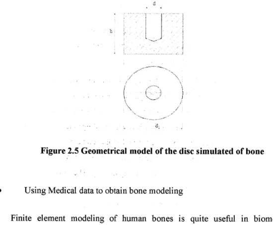
was established as the model of the femur. The height of the disc corresponded with thickness of cortical tissue of femur. The hole corresponding with diameter of the drill

and representing its edge geometry was simulated in the disc (Figure 2 below). The

Inventor Professional 2008 software was applied in order to work out the geometrical models [45].

Figure 2.5 Geometrical model of the disc simulated of bone

• Using Medical data to obtain bone modeling

Finite element modeling of human bones is quite useful in biomechanical simulations. Finite element analysis is the most appropriate technique for analyzing mechanical properties of the complex human bone structure. Due to the availability of low cost computing power, three-dimensional analysis and investigation of any complex structure can be done in virtually in no time. Human bone FE models are generated from image data obtained from medical scanning systems like MRI or CT.

Three-dimensional (3D) finite element (FE) stress analysis provides a complete description of the stress field in a bone structure. To some, this information is a key factor for understanding bone functional behaviour in many research and clinical applications. For Example, fracture risk assessment, design and validation of prosthetic implants, are the possible applications of the 3D FE analysis in clinical studies. The bone structures depends on their shape and size, as well as on the mechanical properties of the material of which they are composed [46]

There are several method used from medical data to build the bone modelling in

FE; using Computed tomography (CT) scan and Magnetic Resonance Imaging (MRI)

scan.

• Using Computed tomography (CT) data obtain from real bone

Finite element analysis (FEA) is widely adopted to investigate the mechanical behaviour of bone structures. Computed tomography (CT) data are frequently used to

generate FE models of bone. If properly calibrated, CT images are capable of providing accurate information about the bone morphology and tissue density.

In the early period the methods used to derive bone geometry and mechanical properties were inaccurate and sometimes highly invasive and destructive. More recently, Marom et al. [47] pointed out many ofthe advantages ofusing computerised tomography (CT) scans in bone modelling. CT images provide accurate information about bone geometry, the radiographic density (RD) reported in the CT images can be related to the mechanical properties of bone, and moreover CT scanning is a mildly invasive routine diagnostic method which permits the modelling of human bones in vivo. CT systems have the capability ofmeasuring the linear attenuation ofthe tissues

under examination.

Generation of subject-specific finite element (FE) models from computed

tomography (CT) datasets is of crucial for application of the FE analysis to bone

structures. However, a great challenge remains is the automatic assignment of bone

material properties from CT Hounsfield Units into finite element models. The

researcher [48] proposes a new assignment approach, in which material properties are

directly assigned to each integration point. Instead of modifying the dataset of FE

models, it divides the assignment procedure into two steps: generating the data file of

the image intensity of a bone in a MATLAB program and reading the file into

ABAQUS via user subroutines. Its accuracy has been validated by assigning the

density ofa bone phantom into a FE model. The proposed approach has been applied

to the FE model of a sheep tibia and its applicability tested on a variety of element

types. The proposed assignment approach is simple and illustrative. It can be easily

modified to fit users' situations.

In another works they develop a special program that can read a CT data set as well as the FEA mesh generated from it, and assigning each element of the mesh the material properties derived from the bone tissue density at the element location. The program was tested on phantom data sets and was adopted to evaluate the effects of the discrete description of the bone material properties. A three-dimensional FE model was generated automatically from a 16 bit CT data set of a distal femur acquired in vivo. The strain energy density (SED) was evaluated for each model element for increasing model complexity (number of different material cards assigned to the model). The computed SED were strongly dependent on the material mapping

strategy.

Computed tomography (CT) represents, at present, the method of choice for the generation of these subject-specific finite-element models, since from CT data it is possible to define the geometry and the local tissue properties of the bone segment to be modelled. However, the data processing techniques used to extract this information from the CT data may frequently be affected by non-negligible errors that propagate in an unknown way through the various steps of the model generation, affecting in an unpredictable way the accuracy of the model predictions.

In many studies the density information provided by the CT dataset is used to derive an inhomogeneous, although locally isotropic, the distribution of the bone tissues mechanical properties. This procedure involves two steps. At first the CT data are calibrated to correlate the Hounsfield units to the apparent or to the ash density of the bone tissue. This step is sometimes performed using a calibration phantom [49- 53], or assuming conventional values derived from literature for selected regions [54].

In both cases the obtained density values cannot be assumed to be error-free. Then the density of the bone tissue is related to its Young's modulus, or to its strength, using empirical equations based on experimental measurements. The coefficients of these equations are affected by an uncertainty due to the significant scattering of these experimental measurements [55-58].

However, using the proposed method to build a finite-element model of a femur from a CT dataset, of a quality usually achievable in the clinical practice, the variation coefficients of the output variables never exceed 9%. This uncertainty on the results seems admissible since these models are commonly used in the orthopaedics research to discriminate between conditions involving much larger differences. Furthermore, the uncertainties related to the boundary conditions definition in the generation of a subject-specific finite- element model of a bone segment are definitely far higher.[59]

Rough

Figure 2.6 Assigning material properties i.e. density from CT scan of bone to FE bone model [60]

• Using MRI data obtain from real bone

The medical scanning system gives an accurate measurement of anatomical geometry.

The accurate representation of the anatomically specific geometry in the finite element model enhances its function especially when motion of a joint is of major concern. However, the generation of a suitable finite element model of human body parts with accurate anatomically specific geometry is still a formidable task, especially if hexahedral solid elements are preferred.

40

Conventional methods adopted in existing FE modeling packages are very time consuming and not suitable for modeling of human bones. So compared to the computational time, the effort needed to generate the finite element model generally dominates the overall process time.

A technique is developed to make FE model of bones from MRI7CT scan data [61]. This technique is a modification over conventionally used techniques. In conventional technique solid modeling processes intermediate solid / surface generation is essential before getting finite element model from the scan data. If this necessity is eliminated, process time and steps are shortened. Conventional process for finite element meshing from MRI scan data requires two intermediate steps first interior and exterior contour point extraction of bones and second solid modeling from contour data extracted. An algorithm is developed and implemented to obtain a meshed model of bones directly from the contours. This technique is developed and implemented to obtain FE meshes from Magnetic Resonance Imaging (MRI) / Computed Tomography (CT) scan data.

Other studies [62] use finite element analysis of the tibia to evaluate stresses developed in the tibia under static loads and to study the effect of varying material properties on these stresses. A 3-D solid model of the human tibia and the fibula was constructed using Magnetic Resonance Imaging and solid modeling software.

Loading conditions and material properties used were taken from the literature. Two finite element models were taken into consideration. A model of the tibial post up to a length of 130 mm was studied to compare results to previous literature and a model of the whole tibia under similar loading conditions was analyzed. This model of the tibia proved to be extremely accurate and could be used to study the behavior of the tibia under further varying properties of cancellous bone and under various loading conditions. Moreover, viscoelastic properties of compact bone could be applied to this model. The effect of muscle forces and the fibula on stresses developed would be of extreme interest. This would definitely seem to reduce the deflection of the tibia reported in this study. The geometric characteristics which play a very important part on stresses developed have been captured extremely accurately.

2.7 Experimental Approach

This section discusses the selection of experimental approached done by previous literature studies. It consists of sample preparation, detail on how the sample of the drilled bone was prepared and the selection of material that may exhibit similar properties to bovine bone. The method of temperature measurement during the drilling procedure were also discussed.

2.7.1 Properties of bone

Bone is a porous non-homogeneous material; different location would give variation in the structural density, which would result inherent fluctuation in the drilling temperature. The temperature profile of a material depends on the specific heat capacity and on thermal conductivity. Thermal gradient exists when there is a two different temperature. Thus, heat is transferred and will continue to transfer as long as there is temperature gradient, when these two regions are equal, the specimen is in a state of equilibrium. However, when biological tissues are exposed to heat in drilling, the temperature equilibrium is not achieved, as the exposure times are usually too short. When the temperature reached the non-equilibrium state for the short exposures, it is known as a function of the exposure temperature and time, and the specific heat capacity being constant [63]. Cowin SC. [64] and Kohles SS. [65]

states that bone has mechanical properties of anisotropic. Hence isotropy of its thermal conductivity must be counted. Davison [66] also supported that bone is to be treated as isotropic

Heat generation during drilling common problem is due to the sensitivity of bone to heat damage and the difficulty of conducting heat away from the cutting edge, both as a result of the poor conductivity of the bone and the inability to use a coolant because of the danger of causing infection to the area. Bone is a poor conductor of heat, with the thermal conductivity of fresh cortical bone in the region of 0.38±2.3 J/msK [67-69]. However, some of the heat generated during drilling may be partly spread out by the presence of blood and tissue fluids and partly carried away by the chips formed.

Table 2.1 Material properties of bone used in FEM

Thermal Conductivity Specific heat Density, kg/m"5 Reference

Human 0.16 to 0.34 W/m°C 1.14 and 2.37 J/gm °C ¹⁹⁰⁰ [70]

Bovine 0.54 W/mK 1260 J/kg K 1800 [66]

PMMA 0.50 W/mK 1297.9 J/kgK 1683 [71]

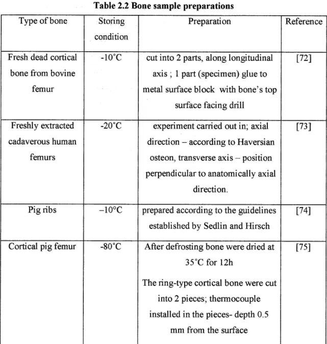
• Sample preparation

Sample preparation may vary from choice of animal and its specific parts to the condition of the bone i.e. wet or dry. Below are some of the summarize sample preparation methods;

Table 2.2 Bone sample preparations Type of bone Storing

condition

Preparation Reference

Fresh dead cortical bone from bovine

femur

-10°C cut into 2 parts, along longitudinal axis ; 1 part (specimen) glue to metal surface block with bone's top

surface facing drill

[72]

Freshly extracted

cadaverous human femurs

-20°C experiment carried out in; axial direction - according to Haversian

osteon, transverse axis - position perpendicular to anatomically axial

direction.

[73]

Pig ribs -10°C prepared according to the guidelines established by Sedlin and Hirsch

[74]

Cortical pig femur -80°C After defrosting bone were dried at

35°C for 12h

The ring-type cortical bone were cut into 2 pieces; thermocouple installed in the pieces- depth 0.5

mm from the surface

[75]

Cattle tibia

Mid-shaft of bovine femora

-18°C

Stored in freezer

Special container holding normal saline solution, fitted with heating

element for solution maintain at 37°C

Wrap in gauze; soaked in mammalian Ringer's solution (mimic physiological fluid) and

Wrapped in resealable bag.

Stored in freezer

[76]

[77]

Researcher conducted various test using cadaveric bone for scientific experimentation

practice. Thus Sedlin and Hirsch [78] have clearly established the importance of

properly harvesting and storing fresh cadaveric bone, in order to preserve its mechanical properties. Mc Elhaney et. al. [79] demonstrated that preservation of cadaveric bone specimens with formalin altered the mechanical properties of these bones, making them potentially unsuitable for quantitative mechanical tests.

• Using Bovine Bone

Some demonstrated that even the time between death and harvesting of specimens may have some effect on the mechanical properties of harvested bone [80].

Fortunately, changes associated with post mortem enzymatic degradationare probably minimal with regard to hard tissues, such as bone. However, it should be remembered that even the best preparation of cadaveric bone would differ from living, in situ bone

in some way.

Properties also vary between the sexes. Investigator found that the drilling temperatures of female bovine tibias are higher compare to the male tibias. This may be due to a higher content of calcium in female bones. The drill speed was found to be a significant parameter on the maximum temperature. Moreover, the maximum temperature increased with an increasing drill tip angle and bone mineral density.

Therefore the bone quality around the drill site was found to be worse than the bone samples exposed to low temperatures [81].