Numerical Simulation of Morning Glory Spillway at Various Discharge Capacity using Lattice Boltzmann Method
by
Nasiha Sofwani Binti Mohamad Shiham 17002838
Dissertation submitted in partial fulfilment of the requirements for the
Bachelor of Civil Engineering with Honours
JANUARY 2022
Universiti Teknologi PETRONAS Bandar Seri Iskandar
32610 Seri Iskandar Perak Darul Ridzuan
i
CERTIFICATION OF APPROVAL
Numerical Simulation of Morning Glory Spillway at Various Discharge Capacity using Lattice Boltzmann Method
by
Nasiha Sofwani Binti Mohamad Shiham 17002838
A project dissertation submitted to the Civil Engineering Programme Universiti Teknologi PETRONAS in partial fulfilment of the requirement for the
BACHELOR OF CIVIL ENGINEERING WITH HONOURS
Approved by,
_____________________
(Dr. Siti Habibah Binti Shafiai)
UNIVERSITI TEKNOLOGI PETRONAS SERI ISKANDAR, PERAK
January 2022
ii
CERTIFICATION OF ORIGINALITY
This is to certify that I am responsible for the work submitted in this project, that the original work is my own except as specified in the references and acknowledgments, and that the original work contained herein has not been undertaken or done by unspecified sources or persons.
__________________________________________
NASIHA SOFWANI BINTI MOHAMAD SHIHAM
iii
ABSTRACT
This research is focused on finding the discharge capacity of the morning glory spillway at the funnel of the pier structure. The software used for this numerical simulation study is MATLAB. Using MATLAB, the result can be guaranteed accurate is effective plus more control over the results compare to other software. Not to mention, MATLAB is a more friendly user for easy and normal simulation. The numerical simulation will be created using the Lattice Boltzmann Method and LABSWETM for the modeling. The parameters to create the model such as discharge rate, velocity, the lattice size, height of the water, density, and the dimension of vortex breaker are collected from previous research related to this project. The model was calibrated through the validation the of model for flow around a cylinder in 2D using LBM. To reduce the vortex formation and the decrease in discharge capacity, two models of piers have been created; piers at 45-degree and 90-degree. The flows around the piers are analyzed and tested in the software. As a result, the graph discharge coefficient against the height of the water is plotted to determine the flow rate increment and decide the best design for the spillway structure.
Keywords: Lattice Boltzmann method, Spillway Morning Glory, Piers, MATLAB, LABSWETM
iv
ACKNOWLEDGMENT
First and foremost, before I thanks all the people involved in giving a contribution to my final year project, I would like to praise Allah the Almighty, Prophet Muhammad (S.A.W), his family, and companies (R.A) for giving me the strength to complete my two semesters of final year project at Universiti Teknologi PETRONAS (UTP).
Nevertheless, the author would like to express her utmost gratitude towards her parents, for it was them who had given the author guidance and moral support required throughout 8 months. The author would also like to take this opportunity to extend her appreciation to all other individuals, both family and friends that have cheered and supported the author during this tough phase. They are the best supporter that she ever had and their prayers are what keep her struggling towards better and keep moving forward in achieving her goals.
Being here was a great opportunity and without certain individuals that help the author go through this journey, she wouldn’t be standing here today. Author special gratitude and acknowledgment goes to the Senior Lecturer from Universiti Teknologi PETRONAS (UTP), Dr. Siti Habibah Binti Shafiai as her supervisor for this project who is willing to spend her time providing support during the entire training period to ensure the author can achieve the objectives of her final year project.
Not to forget, credit to all members of the same group under Dr. Habibah. They cooperated with her by sharing their project content, and knowledge and providing her the virtual support so that I don’t face everything alone. They gave me great exposure to how some tasks could be done and also teach her some new things. Their patience and guidance contributed to several skill developments, knowledge, and self- development towards accomplishing the goals of this final year project.
Last but not least is to author’s friends who fought side by side through hardship and pain together in completing the final year projects. She is glad to have met them and be able to share experiences. They have been a very good listener and friends throughout these 8 months. They continuously supported her and keep giving her boosters whenever she faced any problems. They are one of the reasons that the experience turns out to be a blast because they are always there for her.
v
TABLE OF CONTENT
CERTIFICATION OF APPROVAL ... i
CERTIFICATION OF ORIGINALITY ... ii
ABSTRACT ... iii
ACKNOWLEDGMENT ... iv
TABLE OF CONTENT ... v
LIST OF FIGURES ... vii
LIST OF TABLES ... viii
LIST OF EQUATIONS ... viii
CHAPTER 1 INTRODUCTION ... 1
1.1 BACKGROUND OF STUDY ... 1
1.2 PROBLEM STATEMENT ... 2
1.3 OBJECTIVES ... 3
1.4 SCOPE OF STUDY ... 3
CHAPTER 2 LITERATURE REVIEW ... 4
2.1 INTRODUCTION ... 4
2.2 HYDRODYNAMICS ... 4
2.4 HYDRAULIC FACILITY: DAM ... 6
2.5 AUXILIARY STRUCTURES ... 7
2.5.1 RESERVOIR ... 7
2.5.2 GATES... 7
2.5.4 SPILLWAYS ... 8
2.6 SHAFT SPILLWAYS ... 10
2.6.1 MORNING GLORY SHAFT SPILLWAY ... 10
2.7 FREE VORTEX AT INTAKES ... 11
2.8 LATTICE BOLTZMANN METHOD ... 11
2.8.1 LATTICE BOLTZMANN EQUATION ... 12
2.8.2 LATTICE PATTERN ... 13
2.8.3 LOCAL EQUILIBRIUM DISTRIBUTION FUNCTION ... 15
2.8.4 SGS FOR SHALLOW WATER EQUATIONS ... 16
2.8.5 LABSWETM ... 16
CHAPTER 3 METHODOLOGY ... 18
vi
3.1 PROJECT WORKFLOW ... 18
3.2 TOOLS ... 19
3.3 DATA COLLECTION ... 20
3.4 MODEL VALIDATION ... 22
3.4.1 2D FLOW AROUND A CYLINDER ... 22
3.4.2 THE MATLAB CODING FOR 2D FLOW AROUND CYLINDER ... 25
3.5 PROJECT GANTT CHART ... 27
CHAPTER 4: RESULTS AND DISCUSSION ... 29
4.1 NUMERICAL STUDY OF 2D FLOW OF THE ANTI-VORTEX PIERS AT MORNING GLORY SPILLWAY ... 29
4.1.1 MEASURED DATA ... 29
4.1.2 VELOCITY VECTOR ... 33
4.1.3 MATLAB CODING ... 40
CHAPTER 5: CONCLUSION AND RECOMMENDATION ... 42
CHAPTER 6: REFERENCE ... 43
CHAPTER 7: APPENDIX ... 45
vii
LIST OF FIGURES
Figure 1: Turbulent flow ... 5
Figure 2: Laminar Flow ... 5
Figure 3: Various conditions of hydraulic jump ... 6
Figure 4: Cross-section of Morning Glory Spillway at the intake funnel. ... 10
Figure 5: Structure of Morning Glory Spillway ... 10
Figure 6:Square Lattice ... 14
Figure 7: Hexagon Lattice ... 14
Figure 8: Methodology of flow chart ... 18
Figure 9: MATLAB logo ... 19
Figure 10: The effect of number (left) and angle (right) of Anti-vortex piers in square spillway ... 20
Figure 11: The effect of Anti-vortex piers on flow parameters in submergence threshold ... 20
Figure 12: Comparison Chart of Discharge coefficient and Depth of submergence. 21 Figure 13: The Lattice of 140x42 solid ... 22
Figure 14: Comparison of depth over channel along the centreline for flow around cylinder ... 23
Figure 15: Streamline of 2D flow around cylinder ... 24
Figure 16:Velocity Vector for flow around cylinder ... 24
Figure 17: Lattice solid for pier at angle 45. ... 30
Figure 19:Graph of water level at piers of angle 45... 31
Figure 18: Graph of velocity for piers at angle of 45 ... 31
Figure 20: The Lattice solid for piers at an angle of 90 ... 32
Figure 21: Velocity of piers at an angle of 90 ... 32
Figure 22: Streamline of piers at angle 45 ... 33
Figure 23: Velocity vector for piers at an angle of 45 ... 33
Figure 24: Velocity vector for piers at an angle of 90 ... 34
Figure 25: Streamline of piers at an angle of 90 ... 34
Figure 26: Graph height of water versus discharge coefficient ... 37
Figure 27: Graph height of water versus rate of flow for angle 45-degree ... 37
Figure 28: Graph height of water versus rate of flow for angle 90-degree ... 38
Figure 29: Graph height of water versus discharge coefficient ... 38
viii
Figure 31: Discharge coefficient vs H/D for different models ... 39
Figure 30: Rating curve for different models. ... 39
LIST OF TABLES
Table 1: The parameter for streaming step ... 12Table 2: FYP Ⅰ Gantt chart ... 27
Table 3: FYP Ⅱ Gantt chart ... 28
Table 4: Piers at angle 90-degree ... 35
Table 5. Piers at angle 45-degree ... 36
LIST OF EQUATIONS
Equation 1: Renold number ... 5Equation 2: Streaming step ... 12
Equation 3: Collision Step ... 12
Equation 4: Linear Collision Operator ... 12
Equation 5: Equilibrium distribution function at single state ... 13
Equation 6: Kronecker delta function ... 13
Equation 7:BGK collision operator ... 13
Equation 8: Lattice Boltzmann Equation ... 13
Equation 9: velocity vector ... 14
Equation 10: Na constant after Velocity vector value applied ... 14
Equation 11: LBE for fluid flow simulation ... 14
Equation 12: Equilibrium function... 15
Equation 13: Condition must be followed in shallow water simulation. ... 15
Equation 14:Local equilibrium function ... 15
Equation 15: Turbulence equation for shallow water condition ... 16
Equation 16:Relaxation Time ... 16
Equation 17: Total Viscosity equation ... 16
Equation 18: Strain-rate Sensor ... 16
Equation 19: Total Relaxation Time ... 17
Equation 20: Eddy Relaxation Time ... 17
Equation 21 : Discharge coefficient ... 34
1
CHAPTER 1 INTRODUCTION
This chapter highlights the explanation of the project title and provides clarification on the expected outcome of the project that comprises the background of the study, problem statement, objectives, and scope of the project research study. The background of the study discusses the purpose of the Morning Glory Spillway for dam operation. The problem involved with the current situation and condition of the study will be discussed further. The objectives and scope of the project are laid out as the guideline to complete the project
1.1 BACKGROUND OF STUDY
The Morning Glory Spillway is a roofed conduit that conveys flow from one level to another rapidly. Although this sort of spillway is comparable to a siphon spillway, it behaves differently. These spillways are used to manage erosion of structures and highway culverts in addition to dams. In dams with steep abutments across narrow valleys or a diversion tunnel to transfer water flow downstream of the dam, this form of the spillway is economically efficient. Furthermore, morning glory spillways in stormwater drainage systems or water conveyance systems convey flows from upstream to downstream (from the catchment basin to the tunnel drainage system in hilly places). Morning glory spillways are used in these situations, together with
“vortex basins,” which give the flow an angular velocity, resulting in a circling flow in the glory hole. Morning-glory spillways are standing structures within the dam reservoir that play a critical role in the dam's operation. During a flood, the continual weight and hydrodynamic loading on the body of the spillway concrete structure complicate the structure-fluid interaction study.
2
A fluid-structure interaction analysis with coupled computational fluid dynamics and structural analysis can accurately simulate the performance of these spillways during overflow. Therefore, the preferable method of understanding and designing would be analysis through the hydraulic model for the structure.
1.2 PROBLEM STATEMENT
The study of fluids in motion or at rest is known as hydraulics. The study of fluids in motion is known as hydrodynamics, while fluid properties in static equilibrium are known as hydrostatics (motionless). In designing hydraulic structures, it is important to fully understand and analyze the flow characteristics passing through these structures. For instance, spillways are provided for storage, multipurpose, and detention dams to release excess water or flood water that cannot be contained in the designated storage space, as well as diversion dams to bypass flows that have been turned (redirected) into the diversion system. The significance of a safe, reliable spillway cannot be overstated; many dam catastrophes have been driven by spillways that were inadequately built and/or constructed or spillways with insufficient discharge capacity. Vortices can occur at many types of hydraulic structures, such as hydropower intakes, spillway intakes, or pump sumps which can hurt the structure's operation. A vortex is a turbulent flow of fluid that is spinning and has a closed streamline. In particular, the morning glory spillway operates in a free mode with radial and axial velocity, allowing water to flow directly into the spillway. However, during the vortex phenomenon, incidence and tangential velocity cause the flow path to diverge from the direct mode and travel a longer path, resulting in energy loss and a reduction in discharge capacity.
3
1.3 OBJECTIVES
• To develop and model the simulation using the Lattice Boltzmann Method.
• To analyze and test the discharge capacity of swirling flow at the intake funnel of Morning Glory Shaft Spillway at various data.
• To propose the design of a compatible spillway with suitable discharge capacity
1.4 SCOPE OF STUDY
The scope of the study for this project will focus on the various discharge capacity at the intake funnel of Morning Glory Spillways. As for the design of the spillway rotational flow, the numerical simulation will be created using the Lattice Boltzmann Method and LABSWETM for the modeling. After the hydrodynamic flow has been determined, the data will be analyzed to recommend the best structure design for the shaft spillway which can avoid the formation of the vortex and maintain the discharge capacity.
4
CHAPTER 2 LITERATURE REVIEW
2.1 INTRODUCTION
This chapter will describe the literature collected that is related to the project matter.
The topic that will include in this chapter is Hydrodynamics, Hydraulic facilities such as dams, reservoirs, and spillways. More detailed information will be enlightened on the spillway’s topic about the project’s main chosen structure which is Morning Glory Shaft Spillway. Not forgetting the Lattice Boltzmann method and its components, the backbone of this whole trial.
2.2 HYDRODYNAMICS
Fluid mechanics is the study of science that deals with the mechanical properties of fluids when forces are exerted upon them. It's a field of classical physics with practical uses in hydraulics and aeronautics, chemical engineering, meteorology, and zoology. Water is recognized as the most familiar fluid and the study regarding it is widely known as hydrostatics, the science of water at rest, and hydrodynamics, the science of water in motion. According to McGraw-Hill (2005), Hydrodynamics is the study of a fluid and the interaction of the fluid with its boundaries, especially in the incompressible inviscid case.
The study of hydrodynamics is concerned with the physical conservation laws of mass, momentum, and energy. These principles can be expressed mathematically in either integral or differential form. The integral form is beneficial for large-scale investigations because it delivers solutions that are sometimes excellent and sometimes not but are always valuable, especially in engineering applications. For small-scale analysis, the differential form of the equations is preferred.
5
Although differential forms can theoretically be utilized for any issue, exact solutions are only available for a restricted number of various flows. The majority of problems require the use of numerical methods to solve. Hydrodynamics is used to examine closed-conduit and open-channel flow, as well as to calculate forces on submerged bodies. Experimental and theoretical research on flow in closed conduits, or pipes, has been substantial.
Renold Number = 𝑉𝐷𝜌 𝜇 Equation 1: Renold number
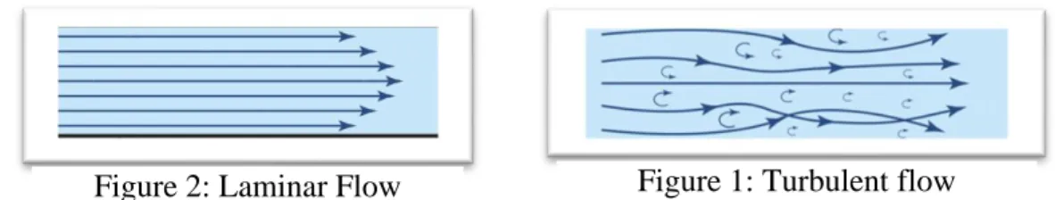
Based on the Reynolds number given by the equation, where V is the average velocity and D is the pipe diameter, is less than about 2000, the flow in the pipe is laminar. In this case, the solution to the continuity, momentum, and energy equations is readily obtained, particularly in the case of steady flows. If ReD is greater than about 4000, the flow in the pipe is turbulent, and the solution to the continuity, momentum, and energy equations can be obtained only by employing empirical correlations and other approximate modeling tools. The ReD region between 2000 and 4000 is the transition region in which the flow is intermittently laminar and turbulent.
The bottom slope and water depth change with position in most open-channel flows, and the free surface is not parallel to the channel bottom. The flow is called a gently varied flow when the slopes are small and the variations aren't too abrupt. A differential equation for the rate of change of the water depth concerning distance along the channel is derived from an energy balance between two portions of the channel. The shape of the water surface is determined by solving this equation, which can be done using any of the many numerical approaches available.
FIGURE 1: Laminar Flow Figure 2: Laminar Flow Figure 1: Turbulent flow
6
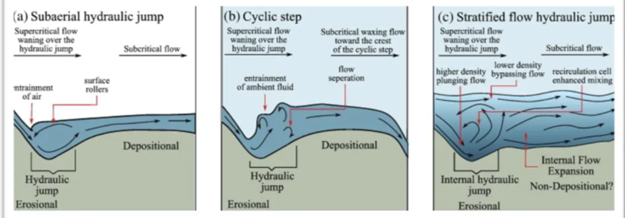
Rapidly fluctuating flows include flow over spillways and weirs, as well as flow over a hydraulic jump. The fluctuations in water depth with distance along the channel are substantial in these circumstances. The pressure distribution with depth may not be hydrostatic in this situation due to the enormous accelerations, as it is in the case of progressively varying and homogeneous flows. Approximation techniques are used to solve problems with rapidly varying flows.
2.4 HYDRAULIC FACILITY: DAM
A dam is a structure that is built to store water across a stream, a river, or an estuary. They are built for drinking water, irrigation scorched, and semiarid lands, or industrial developments. The huge amount of water retained in the reservoir would be used to generate hydroelectric power, to lower the peak discharge of floodwater during heavy storms or snowmelt, or to upsurge the water depth in the river for navigation of ships and barges to transport more easily. Dams can help in recreating a lake for activities like swimming, boating, and fishing. The dam is usually built for more than one purpose and they were helping to properly function by spillways, movable gates, and valves that navigate the release of surplus water downstream of the dam. There are also intake structures that help in conveying the water to the far-distant place from the dam’s location through the designated canals, tunnels, or pipelines.
In a multipurpose scheme designed, a dam acts as the central structure to retain the water resource on a provincial origin. For the developing countries, the multipurpose dams play a critical role in the operation while a single purpose dams give benefits to the industries such as agriculture development, hydroelectric power production, and general industrial growth. Regrettably, the construction of these
Figure 3: Various conditions of hydraulic jump
7
hydraulic structures become a debate in the environmental concern due to the impact of migrating fish and riparian ecosystems, especially the large reservoir which can overwhelm a vast land that homes many living creatures and plants.
In Engineering terms, dams are classified based on their structural types and construction materials. The conclusion in determining the type of dam built mostly depends on the foundation characteristic of the valley, the availability of building materials, the limitation of transporting network from the site, and the experiences of the engineers respond to the project. Nowadays, the common materials usually in between of concrete, earth fill, and rockfill. While in the past, few numbers of dams were created by joined masonry which in the present-day exchanged to the concrete materials. Example of concrete dams is massive gravity dams, thin arch dams, and buttress dams. Embankment dams are including then rockfill and earth-fill dams due to the forms of huge mounds of earth and rock imprinted in the man-made embankments.
2.5 AUXILIARY STRUCTURES
2.5.1 RESERVOIR
Modern engineers have realized the importance of addressing possible reservoir maintenance issues early on. Sediment in rivers has a significant impact on the reservoir's useful life and, as a result, the dam's financing. Because the reservoir has filled with silt, some contemporary dams have become worthless for storing water.
Many others have seen significant reductions ineffective storage capacity. The heavy silt-laden floodwater is permitted to pass through the sluices at the Nile barrages, allowing only the cleaner water to be held at the end of the flood season.
2.5.2 GATES
The opening through dams is needed for the irrigation and water supply, which can maintain the minimum flow in the river for the riverbank interests downstream, electricity generation, and water and silt removal from the reservoir. The gates are
8
constructed by filling the coarse screens at the upstream ends to avoid the incoming of floating and submerged debris. Gates come in a variety of shapes and sizes. The most basic and oldest type is a vertical-lift gate, which may be raised by sliding or rolling against guides and allowing water to pass underneath. The mechanism of radial or tainted gates is similar, but the vertical part is curved to better resist water pressure.
Tilting gates have flaps on their lower edges that are held in place by hinges, allowing water to pour over the top when they are lowered.
Drum gates can autonomously manage the reservoir level upstream to precise levels without the use of mechanical motion. A molded caisson is kept in place by hinges installed on the dam's crest and anchored in a flotation chamber built directly downstream of the crest in one drum gate design. The rotational equilibrium of the caisson is sustained by water pressure in the reservoir and buoyancy in the flotation chamber. The caisson rotates in the same direction as the water level in the flotation chamber, reducing or increasing the flow from the reservoir over the gate. The float controller in the reservoir can be linked to this action and operated automatically.
2.5.4 SPILLWAYS
Spillways are constructed either within a dam or in the side-line of the reservoir to properly release the excess floodwater during flood flows from the reservoir before it overtops the dams. In normal conditions, excess water is reserved from the top of the reservoir and conveyed back into the river through an artificially designed waterway. However, there is some consideration taken where the water may be diverted to an adjacent river valley. The spillway must be hydraulically adequate and structurally safe, as well as placed such that out-falling flows into the river do not damage or undermine the dam's downstream toe. The spillway's surface should also be able to withstand erosion or scouring caused by the extremely high velocities created during a flood's passage through the spillway.
Flood water discharged over the spillway must flow down a channel from a higher elevation at the reservoir surface level to a lower elevation at the natural river level downstream. An energy dissipation mechanism is normally installed near the bottom of the channel, where the water rushes out to meet the natural river, to eliminate the majority of the energy of the flowing water. These devices, also known as Energy
9
Dissipators, are necessary to prevent the river surface from being dangerously scraped by the out falling water's impact. Some projects, such as the Indira Sagar Dam on the Narmada River, include two sets of spillways: main and auxiliary. The main spillway, often referred to as the service spillway, is the one that is used to pass the bulk of the design flood. The auxiliary spillways' crest levels are usually higher, and thus their discharge capacities are smaller. They are activated when the river discharge exceeds the main spillway's capacity.
The capacity of a spillway is usually worked out based on a flood routing study.
As such, the capacity of a spillway is seen to depend upon the following major factors:
• The inflow floods
• The volume of storage provided by the reservoir
• Crest height of the spillway
• Gated or ungated
The volume of the reservoir at various elevation heights, as well as the level of the crest, has an impact on the spillway capacity. The discharging water (Q) is determined by the gate opening if the spillway is gated; thus, the relationship between Q and reservoir water level is different if the spillway is not gated. In most practical situations, however, spillways are equipped with gates, which operate according to a pre-programmed sequence based on the inflow discharge. As a result, when planning a spillway capacity, not only the inflow hydrograph but also the gate operation sequence must be taken into account.
Spillways are typically categorized based on their most noticeable feature, whether that feature is related to the control, the discharge channel, or another component. The following are the most prevalent types of spillways:
• Free Overfall (Straight Drop) Spillway
• Overflow (Ogee) Spillway
• Chute (Open Channel/Trough) Spillway
• Side Channel Spillway
• Shaft (Drop Inlet/Morning Glory) spillway
• Tunnel (Conduit) spillway
•
Siphon spillway10
2.6 SHAFT SPILLWAYS
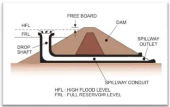
Water enters a Shaft Spillway through a horizontally positioned lip, drops through a vertical or sloping shaft, and then flows to the downstream river channel through a horizontal or nearly horizontal conduit or tunnel. An overflow control weir, a vertical transition, and a closed discharge channel are the three elements that make up the construction.
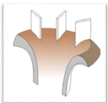
2.6.1 MORNING GLORY SHAFT SPILLWAY
The structure is known as a Morning Glory Spillway when the intake is funnel- shaped. The name comes from the same-named flower, which it resembles quite similarly, especially when fitted with antivortex piers. These piers or guiding vanes are frequently required to reduce vortex action in the reservoir; nevertheless, if the air is permitted to the shaft or bend, it may generate explosive violence in the discharge tunnel unless it is well built for free flow.
The drop intake spillway's discharge characteristics may change depending on the head range. The flow pattern would shift as the head increased, from weir flow over a crest to tube flow, and finally to pipe flow in the tunnel. At relatively low heads, this style of spillway achieves maximum discharging capacity. Should a flood bigger than the selected inflow design flood occur, however, there is little gain in capacity above the intended head? A drop intake spillway can be beneficial at dam sites that are located in narrow gorges with steeply rising abutments. It could also be used in situations where a diversion tunnel or conduit is available.
Figure 5: Structure of Morning Glory Spillway
Figure 4: Cross-section of Morning Glory Spillway at the intake funnel.
11
2.7 FREE VORTEX AT INTAKES
Vortices that occur at many types of hydraulic structures, such as hydropower intakes, spillway intakes, or pump sumps, can harm the structure's operation. Vortices arise at the hydraulic intake structure due to their location relative to surrounding boundaries and geometric qualities, and they originate in a whirling flow. A swirl is a tendency for water at the intake to twist or spin in a twisted or whirling motion. The swirl motion isn't a problem in and of itself. The degree of swirl motion, on the other hand, is what defines the adverse effect and tendency of vortex formation. A vortex is a spinning turbulent flow or fluid with a closed streamline, according to the definition.
These two concepts (swirl and vortex) are connected, and a vortex is a fluid swirling rapidly around a central point.
2.8 LATTICE BOLTZMANN METHOD
The lattice Boltzmann method (LBM) is a new numerical methodology that is particularly efficient and versatile for simulating various flows within complex/varying geometries. It is derived from the lattice gas automata (LGA) to overcome the shortcomings of the LGA. The LBM's fundamental equation turns out to be a discrete variation of the continuum Boltzmann equation in statistical physics, making it self-explanatory. On a macroscopic level, the approach provides a proper average description of fluid while giving the microscopic picture of particle movement in an extremely simplified manner. There are only 3 tasks involved, which are the Lattice Boltzmann equation, lattice pattern, and local equilibrium distribution function.
12 2.8.1 LATTICE BOLTZMANN EQUATION
The Lattice Boltzmann Equation (LBE) applies to a wide range of fluid flows, including shallow water flows. There are two steps involved in the origin of the Lattice Boltzmann Method (LBM), which are a collision step and a streaming step. During the streaming steps, in the direction of their velocities, the particles migrate to the neighbouring lattice points which are conducted by
𝑓𝛼(𝑥 + 𝑒𝛼∆𝑡 , 𝑡 + ∆𝑡) = 𝑓′𝛼(𝑥, 𝑡) + ∆𝑡
𝑁𝛼𝑒2𝑒𝛼𝑖𝐹𝑖(𝑥, 𝑡) Equation 2: Streaming step
Formula Descriptions
𝑓𝛼 Distribution function of particles
𝑓′𝛼 Value of 𝑓𝛼
𝑒 = ∆𝑥 ∆𝑥⁄ Lattice size
∆𝑥 Time step
𝐹𝑖 Force component in the 𝑖-direction
𝑒𝛼 velocity vector of a particle in the α link 𝑁𝛼= 1
𝑒2 ∑ 𝑒𝛼 𝛼𝑖𝑒𝛼𝑖 Constant
Table 1: The parameter for streaming step
While in the collision step, according to scattering laws, the arriving particles at the sites interact with one another and change their velocity directions which govern by
𝑓′𝛼(𝑥, 𝑡) = 𝑓𝛼(𝑥, 𝑡) + 𝛺𝛼[𝑓(𝑥, 𝑡)]
Equation 3: Collision Step
Collision operators control the speed of changes in distribution function particles during the collision. After expanding into the equilibrium state and implying the local equilibrium distribution function to approximate zero, Linear Collision Operator is obtained.
𝛺𝛼(𝑓) ≈ 𝜕𝛺𝛼(𝑓𝑒𝑞)
𝜕𝑓𝛽 (𝑓𝛽− 𝑓𝛽𝑒𝑞) Equation 4: Linear Collision Operator
13
Assume local equilibrium distribution function to an equilibrium state at a single rate.
𝜕𝛺𝛼(𝑓𝑒𝑞)
𝜕𝑓𝛽
= − 1 𝜏 𝛿
𝛼𝛽Equation 5: Equilibrium distribution function at single state
and the range value of 𝛿𝛼𝛽 is taken from:
𝛿𝛼𝛽 = {0,
1, 𝛼 ≠ 𝛽, 𝛼 = 𝛽,
Equation 6: Kronecker delta function
Using the range, input back the value into linear collision operator and become the BGK Collision equation.
Ω𝛼 = −1
τ(𝑓𝛼− 𝑓𝛼𝑒𝑞) Equation 7:BGK collision operator
Finally, the combined equation of streaming and collision steps. Thus, Lattice Boltzmann Equation (LBE) is produced.
𝑓𝛼(𝑥 + 𝑒𝛼∆𝑡 , 𝑡 + ∆𝑡) − 𝑓𝛼(𝑥, 𝑡) = − 1
𝜏𝑡(𝑓𝛼− 𝑓𝛼𝑒𝑞) + ∆𝑡 𝑁𝛼𝑒2𝑒𝛼𝑖𝐹𝑖 Equation 8: Lattice Boltzmann Equation
2.8.2 LATTICE PATTERN
The lattice pattern provides 2 functions for the LBE which are to illustrate the grid points and to govern the movement of the particles. For 2D dimension. the lattice pattern has been classified into two types; square lattice (Figure 14) and hexagon lattice (Figure 15). The models are determined by the number of particles speed at the lattice nodes such as 4-speed, 5-speed, 8-speed, or 9-speed model for square lattice while 6-speed or 7-speed model for hexagon lattice. In every lattice pattern model,
14
lattice symmetry is essential for the repossession of the correct flow equation which can be proven via theoretical analysis and numerical study.
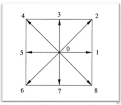
After numerous recent studies and trials, 9-speed square lattice had chosen as the best lattice pattern as it provides accurate results compared to based hexagon in numerical simulations. Figure 16 shows the velocity vector for a 9-speed square lattice. Nodes 1- 8 indicate the movement of the particles at one lattice unit on its velocity while Node 0 represents the rest particle at zero speed.
e
α= {
(0,0), e [cos (α − 1)π
4 , sin (α − 1)π 4 ] ,
√2e [cos (α − 1)π
4 , sin (α − 1)π 4 ] ,
α = 0, α = 1,3,5,7, α = 2,4,6,8.
Equation 9: velocity vector
As mentioned in the LBE before, Nα is the constant in Lattice Pattern and when the velocity value is applied into the equation, and the new LBE equation is;
𝑁𝛼 = 1
𝑒2 ∑ 𝑒𝛼𝑥
𝛼
𝑒𝛼𝑥 = 1
𝑒2 ∑ 𝑒𝛼𝑦
𝛼
𝑒𝛼𝑦= 6
Equation 10: Na constant after Velocity vector value applied
𝑓𝛼(𝑥 + 𝑒𝛼∆𝑡 , 𝑡 + ∆𝑡) − 𝑓𝛼(𝑥, 𝑡) = −1
𝜏𝑡(𝑓𝛼− 𝑓𝛼𝑒𝑞) + ∆𝑡 6𝑒2𝑒𝛼𝑖𝐹𝑖 Equation 11: LBE for fluid flow simulation
Figure 7: Hexagon Lattice Figure 6:Square Lattice
15
2.8.3 LOCAL EQUILIBRIUM DISTRIBUTION FUNCTION
This task is considered the most substantial in the lattice Boltzmann method. It is used to solve the flow equation using lattice Boltzmann equations. The solution to the 2D shallow water equation can be completed by deriving the correct lattice equilibrium distribution function. However, the preceding flow equation has a few restrictions, therefore another option is to suppose that the equilibrium function can be expressed as a power series in macroscopic velocity.
𝑓
𝛼𝑒𝑞= 𝐴
𝛼+ 𝐵
𝛼𝑒
𝛼𝑖𝑢
𝑖+ 𝐶
𝛼𝑒
𝛼𝑖𝑒
𝛼𝑗𝑢
𝑖𝑢
𝑗+ 𝐷
𝛼𝑢
𝑖𝑢
𝑖Equation 12: Equilibrium function
Nevertheless, there are 3 conditions for the LED function must obey for the shallow water equation, which are
∑ 𝑓
𝛼𝑒𝑞(𝑥, 𝑡) = ℎ(𝑥, 𝑡),
𝛼
∑ 𝑒
𝛼𝑖𝑓
𝛼𝑒𝑞(𝑥, 𝑡) = ℎ(𝑥, 𝑡)𝑢
𝑖(𝑥, 𝑡),
𝛼
∑ 𝑒
𝛼𝑖𝑒
𝛼𝑗𝑓
𝛼𝑒𝑞(𝑥, 𝑡) = 1
2 𝑔ℎ
2(𝑥, 𝑡)𝛿
𝑖𝑗+ ℎ(𝑥, 𝑡)𝑢
𝑖(𝑥, 𝑡)𝑗(𝑥, 𝑡).
𝛼
Equation 13: Condition must be followed in shallow water simulation.
By substituting the preceding equations, the following local equilibrium function is obtained:
𝑓𝛼𝑒𝑞 =
{
ℎ − 5𝑔ℎ2 6𝑒2 − 2ℎ
3𝑒2𝑢𝑖𝑢𝑗, 𝑔ℎ2
6𝑒2 + ℎ
3𝑒2𝑒𝛼𝑖𝑢𝑖 + ℎ
4𝑒4𝑒𝛼𝑖𝑒𝛼𝑗𝑢𝑖𝑢𝑗− ℎ 6𝑒2𝑢𝑖𝑢𝑗, 𝑔ℎ2
24𝑒2 + ℎ
12𝑒2𝑒𝛼𝑖𝑢𝑖 + ℎ
8𝑒4𝑒𝛼𝑖𝑒𝛼𝑗𝑢𝑖𝑢𝑗 − ℎ
24𝑒2𝑢𝑖𝑢𝑗,
𝛼 = 0, 𝛼 = 1, 3, 5, 7, 𝛼 = 2, 4, 6, 8,
Equation 14:Local equilibrium function
16
2.8.4 SGS FOR SHALLOW WATER EQUATIONS
Sub grid-scale stress model is used for turbulence flow. The effect of flow turbulence must be taken into consideration in the flow equations to include turbulence in shallow water flows. Therefore, the equation for the shallow water equation with the effect of turbulent is as derived below;
𝜕ℎ
𝜕𝑡 + 𝜕(ℎ𝑢𝑗)
𝜕𝑥𝑗 = 0,
𝜕(ℎ𝑢𝑖)
𝜕𝑡 + 𝜕(ℎ𝑢𝑗𝑢𝑗)
𝜕𝑥𝑗 = −𝑔 𝜕
𝜕𝑥𝑖(ℎ2
2) + (𝑣 + 𝑣𝑒)𝜕2(ℎ𝑢𝑖)
𝜕𝑥𝑗𝜕𝑥𝑗 + 𝐹𝑖 .
Equation 15: Turbulence equation for shallow water condition
2.8.5 LABSWETM
To describe the Lattice Boltzmann model for shallow water equation with the turbulent modeling (LABSWETM), the momentum equation must consider using the eddy viscosity. Kinematic viscosity can be determined by the relaxation time. If defined the relaxation time (Eq. 16), the total viscosity would also be altered as in Equation 17.
𝝉
𝒕= 𝝉 + 𝝉
𝒆Equation 16:Relaxation Time
𝒗
𝒕= 𝒗 + 𝒗
𝒆Equation 17: Total Viscosity equation
Thus, the solution to the lattice Boltzmann equation will be mention before in Eq. 8.
However, the strain-rate sensor must be known and can be calculated in terms of the distribution function. It can be discovered to be connected to the non-equilibrium momentum flux tensor via the Chapman-Enskog expansion.
𝑆𝑖𝑗 = − 3
2𝑒2ℎ𝜏𝑡 ∆𝑡 ∑ 𝑒𝛼 𝛼𝑖𝑒𝛼𝑗(𝑓𝛼− 𝑓𝛼𝑒𝑞) Equation 18: Strain-rate Sensor
17
Then, the finalized equations after some improvement and derivation.
𝝉
𝒕=
𝝉 + √𝝉
𝟐+ 𝟏𝟖𝑪
𝒔𝟐/(𝒆
𝟐𝒉)√∏ 𝒊𝒋 ∏ 𝒊𝒋 𝟐
Equation 19: Total Relaxation Time
𝝉
𝒆=
− 𝝉 + √𝝉
𝟐+ 𝟏𝟖𝑪
𝒔𝟐/(𝒆
𝟐𝒉)√∏ 𝒊𝒋 ∏ 𝒊𝒋
𝟐
Equation 20: Eddy Relaxation Time
18
CHAPTER 3 METHODOLOGY
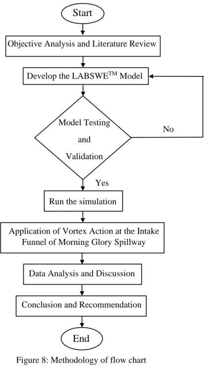
3.1 PROJECT WORKFLOW
Start
Objective Analysis and Literature Review
Develop the LABSWETM Model
Run the simulation
Application of Vortex Action at the Intake Funnel of Morning Glory Spillway
Model Testing and Validation
End
Conclusion and Recommendation Data Analysis and Discussion
No
Yes
Figure 8: Methodology of flow chart
19
3.2 TOOLS
MATLAB is a programming language created by MathWorks. It was originally integrated from a matrix programming language like linear algebra programming and known as matrix laboratory. MATLAB can apply a collaborative setting for numerical computation, visualization, and programming. It made for matrix manipulation;
plotting of function and data; implementation of algorithms; creating user interfaces;
analyzing data and creating models and applications. MATLAB comes with numerous built-in commands and math functions that benefit mathematical calculation, generating plots, and performing the numerical method.
Figure 9: MATLAB logo
20
3.3 DATA COLLECTION
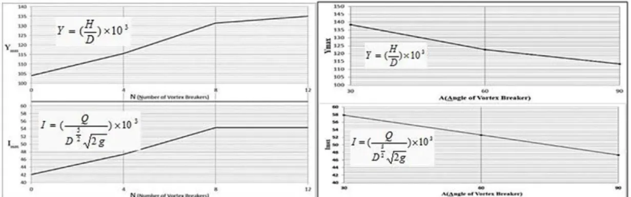
Vortex-breaker is one of the effective methods to control vortex which is used in many dams in order to increase the discharge and discharge coefficient. In the Morning glory spillways, the vortex flow can reduce discharge, discharge coefficient and the performance of spillway. Based on the research done by Kamanbedest. A (2014), the effect angle of vortex breaker and different modes of anti-vortex piers (160 experiments were performed) on discharge coefficient were studied.
According to Kamanbedest. A (2014), Figure 10 indicate that by iincreasing the number of anti-vortex piers increases the inflow and height of water before spillway submerging (increases submergence threshold) and increasing the angle of vortex breaker decreased the passing flow. This represents an increase in the spillway capacity, which increases the risk of severe and dangerous vortexes.
The rise in water height and inflow in the square spillway is 29.8% for water height and 29.2% for inflow in the best mode of utilizing anti-vortex piers, 33.1 percent for water height, and 37.3 percent for inflow in the optimal angle of piers. The results also reveal that in a square spillway without a vortex breaker, the influence of pier Figure 10: The effect of number (left) and angle (right) of Anti-vortex piers in square
spillway
Figure 11: The effect of Anti-vortex piers on flow parameters in submergence threshold
21
angle is greater than the number of piers as shown in Figure 11.. The reason for this is that by deploying a large number of anti-vortex piers as a flow-blocking barrier, the values of Imax and Ymax will be reduced.
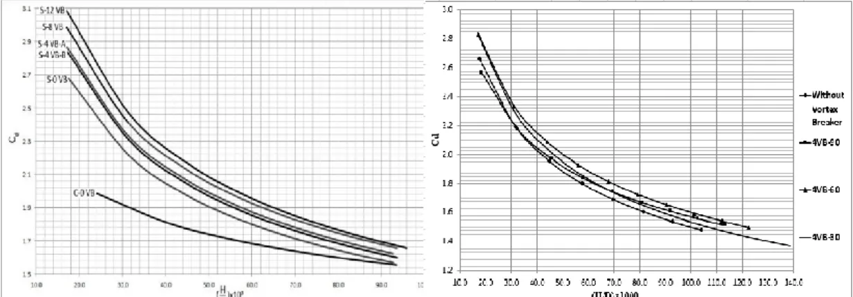
In the Figure 12, Cd and (H/D) values for different modes of number and angle of anti-vortex piers used in square and circular spillways are displayed. For the influence of the number of anti-vortex piers, the maximum discharge coefficient was observed when 12 vortex breakers were placed, and varied patterns of the angle of piers discharge were observed for the influence of the angle of piers.
Figure 12: Comparison Chart of Discharge coefficient and Depth of submergence.
22
3.4 MODEL VALIDATION
3.4.1 2D FLOW AROUND A CYLINDER
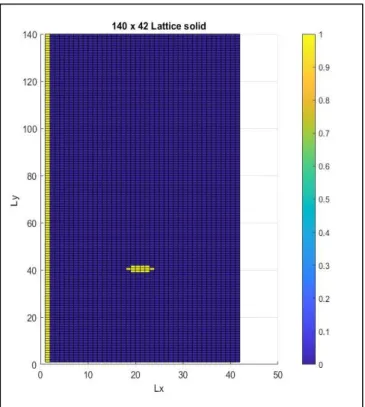
In fluvial hydraulics, flow around a cylinder is a classic problem. It is also a proper test because it reflects a class of flow problems in coastal engineering, such as flow around an island. Referring to (Yulistiyanto 1998), a cylinder with a radius of 0.11m is placed at the center of the channel with the dimension of 4m long and 2m width. The discharge is Q = 0.248 m3/s; outflow depth is h0 = 0.185 m; the bed slope is zb = -6.25 X 10- 4 in the flow direction; and the Manning's coefficient is nb = 0.012.
600 x 300 square lattices were employed in the numerical simulation. T = 1.982, ∆x = ∆y = 0.00667 m, ∆t = 0.00145 s, and τ = 0.00145 s. Along the cylinder's wall, no-slip boundary conditions are used; slip boundary conditions are used for the side walls; the depth at the outflow is set to h = h0; at the inflow boundary, zero gradients for the depth is specified; the inflow velocity u is determined by the discharge; and v = 0 at the inflow boundary. A steady-state solution was found after 40,000 steps. As a result, LABSWETM is utilized to forecast the water surface profile as well as the riverbed topography. Figure 34 shows the lattice solid for the solid profile of 2D flow around the cylinder.
Figure 13: The Lattice of 140x42 solid
23
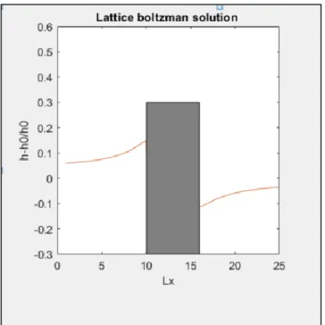
For this section, to describe the numerical results from this project, the following observation is a measured to determine the accuracy and capability of the central scheme. To illustrate them, all subsequent numerical tests include a force term associated with a bed slope such as flow over a bump and flow around a cylinder.
Analytical answers are compared to numerical predictions. Figures 34, 35, and 36 indicate the analysis that is suitable for shallow water equations.
Figure 14: Comparison of depth over channel along the centreline for flow around cylinder
24
Figure 16:Velocity Vector for flow around cylinder
Figure 15: Streamline of 2D flow around cylinder
25
3.4.2 THE MATLAB CODING FOR 2D FLOW AROUND CYLINDER
26
27
3.5 PROJECT GANTT CHART
FYP Ⅰ
TASK WEEK
1 2 3 4 5 6 7 8 9 10 11 12 13 14
Discussion on the project title
Identify the problem Identify the objectives Study on the LBM Study on the MATLAB coding.
Literature review Submit extended proposal
Research on the discharge capacity of morning glory spillway Proposal defense
Review on the research data collection.
Prepared simulation Interim report draft submission
Final submission of the interim report
Table 2: FYP Ⅰ Gantt chart
28
FYP Ⅱ
TASK WEEK
1 2 3 4 5 6 7 8 9 10 11 12 13 14
Literature review
Design numerical model for morning glory spillway
Prepare the simulation Run the simulation and observe the rotational flow
Progress report
submission
Analyses the result and chooses the best hydraulic design of the shaft spillway.
Submission of final report draft
Submission of the final report
Submission of technical report
Prepared dissertation Viva presentation
Table 3: FYP Ⅱ Gantt chart
29
CHAPTER 4: RESULTS AND DISCUSSION
4.1 NUMERICAL STUDY OF 2D FLOW OF THE ANTI-VORTEX PIERS AT MORNING GLORY SPILLWAY
4.1.1 MEASURED DATA
In a numerical model study, the first step is to calibrated the model. It can be done by consider the external factors and the model conditions were taken into observation with regard to the real studies. This research numerical model is performed based on the previous experimental data. The numerical model needs to be calibrated in terms of boundary conditions and simulation. It is vital to acquire steady state in order to get the right and exact data from a numerical model. After examining numerous numerical models, the optimal duration for extracting findings from the model was determined to be 40 seconds in the analyzed numerical model. In the figure below, lattice solid 140x42 is developed as the model for the simulation of piers at the funnel of the morning glory spillway.
In this research, two models of piers at the funnel of the morning glory spillway have been created to find a suitable design for the effective discharge capacity. The limit of the method is restricted to the x-axis and y-axis only. The model of piers was created with the references from circular piano-key Inlet in Shaft Spillways according to the research by Z. Kashkaki, 2018. According to Kam R. Eslinger, 2022, Piano key weirs are straightforward solutions that are as safe and simple to use as standard free-flow spillways while being far more efficient. They have the potential to double the specific flow, significantly lower the cost of most new dams while ensuring their safety, enhance the storage capacity of many existing reservoirs, improve flood management at many existing dams, and raise the overflowing capacity of many existing dams.
30
The channel dimension for the research is; Length (4m), width (0.75m), density is 𝜌 = 1000𝑘𝑔/𝑚3, Renold number, 𝑅𝑒𝐷 = 3.2 𝑥 104 and the time interval of 20sec. the two angles that were consider in this research are: angle of 45ᵒ and 90ᵒ .
Based on figure 16 and figure 17, the water level near the piers of angle 45 is overflowing the structure and thus velocity is depth on the side channel rather than on the centerline of the path. When comparing to the piers at an angle of 90, the velocity shows only a few higher flows at the structure of piers due to the impact of water when reflected a solid wall but goes to a calm state directly after the collision area. These results can be explained more in the next subtopic: Velocity Vector.
Figure 17: Lattice solid for pier at angle 45.
31
Figure 19: Graph of velocity for piers at angle of 45
Figure 18:Graph of water level at piers of angle 45
32
Figure 20: The Lattice solid for piers at an angle of 90
Figure 21: Velocity of piers at an angle of 90
33 4.1.2 VELOCITY VECTOR
The rate of change of an object's position is represented by a velocity vector. The magnitude of a velocity vector indicates an object's speed, whereas the vector direction indicates the object's direction. The principles of vector addition can be used to add or subtract velocity vectors. It also known as the position function's derivative with regard to time. More in-depth velocity field can be observed from Figure 18 and the clear numerical result of streamline can be proved by Figure 19. The velocity vector for both angles shows that the water is drawn to the right-side wall of channel. It can be assumed as the magnitude of water is lower, the direction of water is dispersed to the side of path due to the little force attraction in the originated path and after a while, the flow of water returns to steady state again.
Figure 23: Velocity vector for piers at an angle of 45
Figure 22: Streamline of piers at angle 45
34
According to A. Barati (2014), increasing the angle of piers can leads to the decreasing the inflow and height of water which also indicate that the flow will discharge greater capacity and no risky problems such as decreasing the discharge coefficient and huge swirling vortex will take place. This also produces a good performance of spillway capacity. Table 4 shows the relation between the discharge rate, height of water and the discharge coefficient that calculate using the following equation.
𝐶𝑑 = 𝑄 𝐿 𝑥 𝐻32
Equation 21 : Discharge coefficient
Figure 24: Velocity vector for piers at an angle of 90
Figure 25: Streamline of piers at an angle of 90
35
In order to get more accurate numerical results, the data for Discharge, height of water and the discharge coefficient of Piers at angle-90 degree are analyze with the same parameters of Piers at angle-45 degree.
Piers at angle 90
no. Q (m3/s) H (cm) Cd
1 0.480 0.428 0.428
2 0.473 0.426 0.425
3 0.466 0.424 0.421
4 0.459 0.422 0.419
5 0.452 0.419 0.416
6 0.446 0.417 0.414
7 0.439 0.414 0.413
8 0.433 0.410 0.412
9 0.426 0.407 0.411
10 0.420 0.403 0.411
11 0.414 0.398 0.412
12 0.409 0.394 0.413
13 0.403 0.389 0.415
14 0.397 0.384 0.418
15 0.392 0.379 0.421
16 0.386 0.373 0.424
17 0.381 0.367 0.429
18 0.376 0.361 0.434
19 0.371 0.354 0.441
20 0.367 0.346 0.450
21 0.367 0.346 0.450
Table 4: Piers at angle 90-degree
36
Piers at angle 45
no. Q (m3/s) H (cm) Cd
1 0.031 0.117 0.192
2 0.030 0.116 0.191
3 0.030 0.116 0.190
4 0.030 0.116 0.189
5 0.030 0.116 0.188
6 0.029 0.116 0.187
7 0.029 0.115 0.186
8 0.029 0.115 0.185
9 0.029 0.115 0.184
10 0.029 0.115 0.183
11 0.028 0.115 0.183
12 0.028 0.115 0.182
13 0.028 0.115 0.182
14 0.028 0.115 0.181
15 0.028 0.115 0.181
16 0.028 0.115 0.181
17 0.028 0.114 0.180
18 0.028 0.114 0.180
19 0.028 0.114 0.180
20 0.028 0.114 0.180
21 0.028 0.114 0.180
Table 5. Piers at angle 45-degree
37
Figure 26: Graph height of water versus discharge coefficient for angle 45-degree
Figure 27: Graph height of water versus rate of flow for angle 45-degree
0.170 0.175 0.180 0.185 0.190 0.195
0.117 0.116 0.116 0.116 0.116 0.116 0.115 0.115 0.115 0.115 0.115 0.115 0.115 0.115 0.115 0.115 0.114 0.114 0.114 0.114 0.114
Discharge coefficient
Height of water (m) Graph Cd vs H (angle 45)
0.026 0.026 0.027 0.027 0.028 0.028 0.029 0.029 0.030 0.030 0.031 0.031
0.117 0.116 0.116 0.116 0.116 0.116 0.115 0.115 0.115 0.115 0.115 0.115 0.115 0.115 0.115 0.115 0.114 0.114 0.114 0.114 0.114
Discharge (m3/s)
Height of water (m) Graph Q vs H (angle 45
)
38
Figure 28: Graph height of water versus rate of flow for angle 90-degree
0.000 0.100 0.200 0.300 0.400 0.500 0.600
0.428 0.426 0.424 0.422 0.419 0.417 0.414 0.410 0.407 0.403 0.398 0.394 0.389 0.384 0.379 0.373 0.367 0.361 0.354 0.346 0.346
Discharge (m3/s)
Height of water (m) Graph of Q vs H (angle 90)
0.390 0.400 0.410 0.420 0.430 0.440 0.450 0.460
0.428 0.426 0.424 0.422 0.419 0.417 0.414 0.410 0.407 0.403 0.398 0.394 0.389 0.384 0.379 0.373 0.367 0.361 0.354 0.346 0.346
Discharge coeffiecient
Height of water (m) Graph of Cd vs H (angle 90)
Figure 29: Graph height of water versus discharge coefficient for angle 90-degree
39
Based on Figure (26) to Figure (29), the discharge coefficient for angle 90-degree has greater values compared to angle-45 degree and the spillway produce bigger inflow capacity for 90-degree angle of anti-vortex piers than for 45-degree angle. In simpler words, increasing the angle of anti-vortex pier will increase the inflow capacity and the discharge coefficient values. According to Figure 30, for the constant head, a circular piano key inlet with an angle of 90 degrees overflows a greater quantity of discharge than models with angles of 60 and 45 degrees. When compared to a circular piano key inlet, a shaft spillway with no reformed inlet spills a smaller quantity of discharge. In conclusion, comparison to the shaft spillway, the circular piano key intake performs better. According to the research done by Z. Kashkaki (2019), results showed in Figure 31, that in a constant head, the greater amounts of discharge coefficient have been measured for the circular piano key inlet model with a 90 degrees angle by 15.16%.
Figure 31: Rating curve for different models.
Figure 30: Discharge coefficient vs H/D for different models
40 4.1.3 MATLAB CODING
clear
% main program
% !Input parameters!
length=4;width=0.75;
h0=1.173;he=1.173;v0=0;QinM=1.127;QinT=0.043;
Lx=80;
dt=0.01;max_t=1;
tau=0.500012;gacl=9.81; rou=1000; % fb=0;
tau=1.1; % test laminar flow Cs=0.4;
% !Calculation of parameters!
dx=length/Lx; dy=dx;Ly=width/dy;
e=dx/dt;
%u0=Qin/(h0*(Ly-1)*dy); % h0 should be changed to net h nu_m=(2*tau-1)/6; % molecular viscosity
nu=e^2*dt*(2*tau-1)/6; % kinematic viscosity mu=nu*1000; % dynamic viscosity of water nermax=(Lx-1)*(Ly-1);
Ly=Ly+2;
Xs=1;Xe=Lx;Ys=1;Ye=Ly;
!determine solid values!
% load 'vortex1.mat';
load 'vortex2.mat';
% solid=solid_values(Lx,Ly,a);
% bed data and slope calculation [zb]=bed_data(Lx,Ly,dx,dy);
[Sx,Sy]=bed_slope(zb,Lx,Ly,dx,dy);
% !initialize the depth and velocity field!
for y=1:Ly for x=1:Lx
if solid(x,y)==0 h(x,y) =1.173;
u(x,y)=0.43; v(x,y) = 0;
else
h(x,y) = 0; u(x,y) = 0; v(x,y) = 0;
end end end
ui=u;vi=v;hi=h;
[fb]=fb_distribution(Lx,Ly,dx,dy,h,gacl);
area0=0;
for y = 1:Ly-1
area0 =area0+0.5*(h(1,y)+h(1,y+1))*dy;
end
[ex,ey]=setup(e); % calculate ex and ey
feq = compute_feq(Lx,Ly,h,u,v,e,ex,ey,gacl,solid); % initial feq f=feq; % set initial feq to f
fcon=feq;
iteration=0;
% main loop time=0;
for time=0:dt:200*dt;
iteration=iteration+1;
h_bf=h;
feq = compute_feq(Lx,Ly,h,u,v,e,ex,ey,gacl,solid); % update feq
41
[taut,taue,nue] =
compute_taut(Lx,Ly,solid,tau,Cs,h,e,ex,ey,f,feq,dt); % Large eddy simulation
[fb]=fb_distribution(Lx,Ly,dx,dy,h,gacl);
ftemp =
collide_stream(Xs,Xe,Ys,Ye,solid,taut,gacl,dt,Sx,Sy,u,v,e,ex,ey,feq, f,h,fb); %collide_stream
ftemp=BC_Body_slip(Xs,Xe,Ys,Ye,solid,ftemp,Lx,Ly,fcon,ui,vi,hi,e);
% calculate h,u,v results
[h,u,v,f]=solution(Xs,Xe,Ys,Ye,solid,ftemp,ex,ey);
iteration c = u(50,17)
end
% continuity test
[Q]=continuity(Xs,Xe,Ys,Ye,h,u,dy);
u0=u(50,17);
Fr=u0/sqrt(gacl*he); % Froud Number Re=u0*width/nu; % Renold Number
% !determine solid values!
% function solid=solid_values(Lx,Ly,a) function solid=solid_values(Lx,Ly)
for i=1:Lx for j=1:Ly
if (i-40)^2+(j-21)^2<2.5^2 solid(i,j)=1;
else
% solid(i,j)= a;
solid(i,j)=0;
end end
end
% solid(1:81,1:23)=1; solid(100:Lx,1:23)=1;
solid(1:Lx,Ly)=1;solid(1:Lx,1)=1;
return
42
CHAPTER 5: CONCLUSION AND RECOMMENDATION
As a conclusion, the objective of the research is obtained. The model was able to develop and run the simulation using Lattice Boltzmann method in shallow water.
In the result also mention that the model is tested and able to analyses the discharge capacity of the channel. Among the two proposed piers’ angle, the most suitable angle that proven by this research is piers at angle 90-degree. The real-life case also help this research in properly determining the compatible design for the effective discharge capacity as mention in the scope of this study.
Physical models were used to test an innovative approach named "circular piano-key spillway," which combined the piano-key weir idea with a morning glory spillway. The hydraulic performance of the shaft spillway with no repaired inflow was compared. A Circular piano key spillway with a 90-degree angle demonstrated a higher discharge coefficient than the other models examined in this study. In a geometric comparison of three circular piano-key spillway models, the circular piano- key spillway with a 90-degree angle has the best performance. As a result, increasing their dimension to a certain point improves the discharge coefficient and spillway flow discharge.
For this research, MATLAB was chosen as the software to develop the model.
However, they are more out there that can create better models than these models.
MATLAB was purposely used to develop the lattice Boltzmann models for the shallow water equations (LABSWE and LABSWETM). Based on the simulation done, it suggests that the LABSWETM is accurate and conservative to be used, develop and model the flow of water. However, further study is recommended for this research as the result obtained is little compared to other research regarding the use of LBE in the simulation of shallow flow for the 2D axis.
43
CHAPTER 6: REFERENCE
Amir Abbas Kamanbedast, Seyyed Reza Mousavi, Adel Barati, The Effect of Number and Angle of Guide Piers on Hydraulic Behavior of Morning Glory Spillway with Square Inlet . Adv. Environ. Biol., 8(7), 2377-2383, 2014
B. Yulistiyanto, Y. Zech, and W. H. Graf. Flow around a cylinder: shallow-water modeling with diffusion-dispersion. J. Hydr. Eng., ASCE, 124(4):419-429, 1998.
Enjilzadeh, M. R., & Nohani, E. (2016). Numerical Modeling of Flow Field in Morning Glory Spillways and Determining Rating Curve at Different Flow Rates.
Civil Engineering Journal, 2(9), 448–457. https://doi.org/10.28991/CEJ-2016- 00000048
Faber, T. E. (2019, January 17). fluid mechanics. Encyclopedia Britannica.
https://www.britannica.com/science/fluid-mechanics
hydrodynamics. (n.d.) Collins Discovery Encyclopedia, 1st edition. (2005). Retrieved October 18 2021 from https://encyclopedia2.thefreedictionary.com/hydrodynamics hydrodynamics. (n.d.) McGraw-Hill Concise Encyclopedia of Physics. (2002).
Retrieved October 18 2021
from https://encyclopedia2.thefreedictionary.com/hydrodynamics
hydrodynamics. (n.d.) McGraw-Hill Dictionary of Scientific & Technical Terms, 6E.
(2003). Retrieved October 18 2021
from https://encyclopedia2.thefreedictionary.com/hydrodynamics
hydrodynamics. (n.d.) The Columbia Electronic Encyclopedia®. (2013). Retrieved October 18 2021 from https://encyclopedia2.thefreedictionary.com/hydrodynamics Kashkaki, Z., Banejad, H., Heydari, M., Olyaie, E. (2019). Experimental Study of Hydraulic Flow of Circular Piano-Key Inlet in Shaft Spillways. Journal of