DATA ANALYSIS USING PARTICLE SWARM OPTIMIZATION ALGORITHM
TAI ZU JIE
A project report submitted in partial fulfilment of the requirements for the award of the degree of Bachelor of Engineering (Hons) Electronics Engineering
Faculty of Engineering and Green Technology Universiti Tunku Abdul Rahman
September 2015
DECLARATION
I hereby declare that this project report is based on my original work except for citations and quotations which have been duly acknowledged. I also declare that it has not been previously and concurrently submitted for any other degree or award at UTAR or other institutions.
Signature : _________________________
Name : __TAI ZU JIE______________
ID No. : __11AGB06591____________
Date : __1/9/2015________________
APPROVAL FOR SUBMISSION
I certify that this project report entitled “DATA ANALYSIS USING
PARTICLESWARM OPTIMIZATION ALGORITHM” was prepared by TAI ZU JIE has met the required standard for submission in partial fulfilment of the requirements for the award of Bachelor of Engineering (Hons) Electronics Engineering at Universiti Tunku Abdul Rahman.
Approved by,
Signature : _________________________
Supervisor : Dr. Lai Koon Chun
Date : _________________________
The copyright of this report belongs to the author under the terms of the copyright Act 1987 as qualified by Intellectual Property Policy of Universiti Tunku Abdul Rahman. Due acknowledgement shall always be made of the use of any material contained in, or derived from, this report.
© 2015, Tai Zu Jie. All right reserved.
Specially dedicated to
my beloved grandmother, sister, mother and father
ACKNOWLEDGEMENTS
I would like to thank everyone who had contributed to the successful completion of this project. I would like to express my gratitude to my research supervisor, Dr. Lai Koon Chun for his invaluable advice, guidance and his enormous patience throughout the development of the research.
DATA ANALYSIS USING PARTICLE SWARM OPTIMIZATION ALGORITHM
ABSTRACT
Particle Swarm Optimization (PSO) basically using the method that more tending to social behaviour, for example fish schooling, bird flocking, bees swarming.
This is effective since each particle’s solution seems like know each position and its movement. At the end of the swarming, the particle’s solution supposed to confined to one optimal solution. In this paper, some mathematical function and mechanical components with subject to constraint were introduced to perform optimization using PSO. Furthermore, a modified PSO(Accelerated PSO) were also introduced to compare the results with Basic PSO. Some concern parameters for PSO such as the swarm particle(population size), swarm iterations, self and swarm-confidence factor, weight factor also been introduced in this paper, and have been found the best fitness values for each case problem.
TABLE OF CONTENTS
DECLARATION ii
APPROVAL FOR SUBMISSION iii
ACKNOWLEDGEMENTS vi
ABSTRACT vii
TABLE OF CONTENTS viii
LIST OF TABLES x
LIST OF FIGURES xii
LIST OF SYMBOLS / ABBREVIATIONS xv
LIST OF APPENDICES xvi
CHAPTER
1 INTRODUCTION 1
1.1 Background 1
1.2 Problem Statements 2
1.3 Aims and Objectives 3
2 LITERATURE REVIEW 4
2.1 Optimization algorithms 4
2.1.1 Genetic Algorithm(GA) 4
2.1.2 Simulated Annealing (SA) 5
2.1.3 Evolutionary Algorithm (EA) 7
2.2 Particle Swarm Optimization (PSO) 8
2.2.1 Swarm Intelligence 8
2.3 Unique PSO 9
2.4 PSO Algorithm Flowchart 11
3 METHODOLOGY 12
3.1 Optimization of Rosenbrock function 12
3.2 Optimization of Matyas function 13
3.3 Weight Minimization of Speed Reducer(WMSR) 14 3.4 Weight Cost Minimization of Pressure Vessel (WMPL) 16 3.5 Volume Minimization of Compression Spring (VMCS) 18 3.6 Particle Swarm Optimization (PSO) Algorithm 19 3.6.1 Basic Particle Swarm Optimization (BPSO) 20
3.6.2 Accelerated PSO (APSO) 21
4 RESULTS AND DISCUSSIONS 23
4.1 Optimization of Rosenbrock function 23
4.2 Optimization of Matyas function 29
4.3 Weight Minimization of Speed Reducer (WMSR) 32 4.4 Weight Minimization of Pressure Vessel (WMPV) 39 4.5 Volume Minimization of Compression Spring (VMCS) 46
5 CONCLUSION AND RECOMMENDATIONS 52
5.1 Conclusions 52
5.2 Recommendations 53
5.2.1 Rosenbrock functions 53
5.2.2 Matyas function 54
5.2.3 Weight Minimization of Speed Reducer (WMSR) 54
5.2.4 Weight Minimization of Pressure Vessel(WMPV)54 5.2.5 Volume Minimization of Compression Spring
(VMCS) 54
REFERENCES 55
APPENDICES 57
LIST OF TABLES
TABLE TITLE PAGE
Table 4.1: Comparison results and between BPSO and
APSO algorithms, n= 20 (Rosenbrock). 23
Table 4.2: Comparison results and between BPSO and
APSO algorithms, n=40 (Rosenbrock). 24
Table 4.3: Comparison results and between BPSO and APSO
algorithms, n=60 (Rosenbrock). 25
Table 4.4: Comparison results and between BPSO and
APSO algorithms, n=80 (Rosenbrock). 26
Table 4.5:Comparison results and between BPSO and APSO
algorithms, n=100 (Rosenbrock). 27
Table 4.6:Accuracy results of x and y between BPSO and APSO
algorithms (Rosenbrock). 29
Table 4.7:Comparison results and between BPSO and APSO
algorithms, n=20 (Matyas). 30
Table 4.8: Comparison results and between BPSO and APSO
algorithms, n=40 (Matyas). 30
Table 4.9:Accuracy results and between BPSO and APSO
algorithms (Matyas). 31
Table 4.10:Comparison overall global best between BPSO and APSO algorithms with population, n =20
(WMSR). 33
Table 4.11:Comparison overall global best between BPSO and APSO algorithms with population, n =40
(WMSR). 34
Table 4.12:Comparison overall global best between BPSO and
APSO algorithm with population, n =60 (WMSR). 35 Table 4.13:Comparison overall global best between BPSO and
APSO algorithm with population, n =80 (WMSR). 36 Table 4.14:Comparison overall global best between BPSO and
APSO algorithm with population, n =100 (WMSR).
37 Table 4.15:Comparison overall best solutions(WMSR) by
BPSO, APSO,EA-Coello (WMSR). 38
Table 4.16:Comparison overall global best between BPSO and
APSO algorithm with population, n =20 (WMSR). 39 Table 4.17:Comparison overall global best between BPSO and
APSO algorithm with population, n =40 (WMSR). 40 Table 4.18:Comparison overall global best between BPSO and
APSO algorithm with population, n =60 (WMSR). 41 Table 4.19:Comparison overall global best between BPSO and
APSO algorithm with population, n =80 (WMSR). 42 Table 4.20:Comparison overall global best between BPSO and
APSO algorithm with population, n =100 (WMSR).
43 Table 4.21:Comparison overall best solutions by BPSO, APSO
and EA-Coello algorithm (WMSR). 45
Table 4.22:Comparison overall global best between BPSO and
APSO algorithm with population, n =20 (VMCS). 46 Table 4.23;Comparison overall global best between BPSO and
APSO algorithm with population, n =40 (VMCS). 47 Table 4.24:Comparison overall global best between BPSO and
APSO algorithm with population, n =6 (VMCS). 48 Table 4.25:Comparison overall global best between BPSO and
APSO algorithm with population, n =80 (VMCS). 49 Table 4.26:Comparison overall best solutions by BPSO, APSO
and Coello algorithm (VMCS). 50
LIST OF FIGURES
FIGURE TITLE PAGE
Figure 1.1: Fish schooling which inspired the creation of Particle
Swarm Optimization. 2
Figure 2.1: Evolution flow of genetic algorithm (Copyright Ying-Hong Liao, and Chuen-Tsai Sun, Member,
IEEE) 5
Figure 2.2: Evolution flow of Simulated Annealing (Reference
from intechopen.com) 6
Figure 2.3: Evolution flow of Evolutionary Algorithm
(Reference from
http://www.geatbx.com/docu/algindex-01.html) 7 Figure 2.4: Multi-peaks function as mentioned as above.
(Copyright Swagatam Das) 10
Figure 3.1: Rosenbrock function 13
Figure 3.2: Matyas function 13
Figure 3.3: Speed reducer design actual diagram 14 Figure 3.4: Speed reducer design structure diagram 14 Figure 3.5: Pressure vessel design actual diagram (Reference
from libertyengg.com) 16
Figure 3.6: Pressure vessel design structure diagram 17 Figure 3.7: Tension/Compression Spring actual diagram
(Reference from globalsources.com) 18
Figure 3.8: Tension/Compression Spring structure diagram 18
Figure 4.1: Convergence graph of global optimum, fmin by BPSO and APSO using population size of 20 over
200 iterations. 24
Figure 4.2: Figure 4.1.2: Convergence graph of global optimum, fmin by BPSO and APSO using population size of
40 over 200 iterations (Rosenbrock). 25
Figure 4.3: Convergence graph of global optimum, fmin by BPSO and APSO using population size of 60 over
200 iterations (Rosenbrock). 26
Figure 4.4:Convergence graph of global optimum, fmin by BPSO and APSO using population size of 80 over
200 iterations (Rosenbrock). 27
Figure 4.5: Convergence graph of global optimum, fmin by BPSO and APSO using population size of 100
over 200 iterations (Rosenbrock). 28
Figure 4.6:Elapsed time by simulation of BPSO and APSO
against population size (Rosenbrock). 28 Figure 4.7:Convergence graph of global optimum, fmin by
BPSO and APSO using population size of 20 over
140 iterations (Matyas). 30
Figure 4.8:Convergence graph of global optimum, fmin by BPSO and APSO using population size of 40 over
140 iterations (Matyas). 31
Figure 4.9:Elapsed time by simulation of BPSO and APSO
against population size (Matyas). 31
Figure 4.10:Convergence graph of global optimum, fmin by BPSO and APSO using population size of 20 over
160 iterations (WMSR). 33
Figure 4.11:Convergence graph of global optimum, fmin by BPSO and APSO using population size of 40 over
160 iterations (WMSR). 34
Figure 4.12:Convergence graph of global optimum, fmin by BPSO and APSO using population size of 60 over
160 iterations (WMSR). 35
Figure 4.13;Convergence graph of global optimum, fmin by BPSO and APSO using population size of 80 over
160 iterations (WMSR). 36
Figure 4.14:Convergence graph of global optimum, fmin by BPSO and APSO using population size of 100
over 160 iterations (WMSR). 37
Figure 4.15:Elapsed time by simulation of BPSO and APSO
against population size (WMSR). 38
Figure 4.16:Convergence graph of global optimum, fmin by BPSO and APSO using population size of 20 over
200 iterations (WMSR). 40
Figure 4.17:Convergence graph of global optimum, fmin by BPSO and APSO using population size of 40 over
200 iterations (WMSR). 41
Figure 4.18:Convergence graph of global optimum, fmin by BPSO and APSO using population size of 60 over
200 iterations (WMSR). 42
Figure 4.19:Convergence graph of global optimum, fmin by BPSO and APSO using population size of 80 over
200 iterations (WMSR). 43
Figure 4.20:Convergence graph of global optimum, fmin by BPSO and APSO using population size of 100
over 200 iterations (WMSR). 44
Figure 4.21:Elapsed time by simulation of BPSO and APSO
against population size (WMSR). 44
Figure 4.22:Convergence graph of global optimum, fmin by BPSO and APSO using population size of 20 over
200 iterations (VMCS). 46
Figure 4.23:Convergence graph of global optimum, fmin by BPSO and APSO using population size of 40 over
200 iterations (VMCS). 47
Figure 4.24:Convergence graph of global optimum, fmin by BPSO and APSO using population size of 60 over
200 iterations (VMCS). 48
Figure 4.25:Convergence graph of global optimum, fmin by
BPSO and APSO (VMCS). 49
Figure 4.26:Elapsed time by simulation of BPSO and APSO
against population size (VMCS). 50
LIST OF SYMBOLS / ABBREVIATIONS
BPSO Basic Particle Swarm Optimization APSO Accelerated Particle Swarm Optimization WMSR Weight Minimization of Speed Reducer WMPV Weight Minimization of Pressure Vessel VMCS Volume Minimization of Compression Spring self-confidence factor
swarm-confidence factor
randomness factor for individual best randomness factor for global best velocity of particle at time velocity of particle at time
best position of each particle over time best global solution in the current swarm current best fitness location
initial value of randomness parameter random numbers for APSO
n population size iterations
LIST OF APPENDICES
APPENDIX TITLE PAGE
APPENDIX A: MATLAB codes(BPSO) 57
APPENDIX B: MATLAB codes(APSO) 61
CHAPTER 1
1 INTRODUCTION
1.1 Background
Particle Swarm Optimization (PSO) was published by Kennedy, Eberhart in 1995. He was intended for simulating social behaviour. The method can be used to optimize single/multiple problems iteratively with trying to improve the solution to the best known solutions. The method was inspired by the social behaviour, such as bird-flocking, fish-pooling and bees swarming. Birds or fish trying to do their movement to avoid predators, seek food and mates, optimize environmental parameters such as temperature.
The solution’s particles must be moving with its known velocity within the search space. Every best known solution it’s reach, it will continue search the better best known particle solution. The iteration means that how many times the particle moving to the updated position. Once, the best known solution found, the iteration will be terminated. The iteration could be terminated by settings the parameters.
PSO has many similarities with Genetic Algorithms (GA). PSO optimizes by bounded for solution’s search space and swarm over the space to updated the best known solutions. However, PSO has no evolution operators such as crossover and mutation. PSO has been used widely on several fields, such as machine design, mathematical function optimization, biotechnology, software engineering.
Figure 1.1: Fish schooling which inspired the creation of Particle Swarm Optimization.
1.2 Problem Statements
Why Particle Swarm Optimization is powerful?
PSO method was widely applying on many fields nowadays, This is due to it’s several advantages. One of the advantage that is there are few variable parameters need to be changed compare to GA or other optimization method. The parameters such as lower boundary, upper boundary, population size, iteration. And it doesn’t use the filtering operation such as crossover or mutation.
Furthermore, PSO has better memory capacity than Genetic Algorithm. For the PSO, the particle swarming over a certain iterations, with this, every particle will remembers its own previous best value. The PSO was designed as a artificial intelligence, so it could be applied on various different field such as medical, science, face recognition, mathematics optimization, evolving neural networks to optimize problem.
Moreover, the ability of optimization of PSO will be higher than other optimization algorithms. So, it can be completed the process easily with high speed.
1.3 Aims and Objectives
The objectives of the thesis are shown as following:
i) Data analysis for performing optimization using Particle Swarm Optimization (PSO) by MATLAB software.
ii) Implement and improve data output of the process by using PSO.
iii) Investigate and perform comparison of PSO algorithm with other algorithms.
CHAPTER 2
2 LITERATURE REVIEW
Particle Swarm Optimization was using widely nowadays. Such fields like Science, Medical, Business and Mathematical based are using the systems to optimize it’s own solution. The particles system basically used to optimize the solution within the problem’s search space, and the particles moves around the space to find best solution of certain problems. There have several rules required to be obeyed to optimize problems such as lower boundary, upper boundary, swarm size, iteration of swarming, velocity of swarming. The particles system is basically deals with swarm intelligence.
2.1 Optimization algorithms
Besides PSO, there have some other optimization algorithms were using from previous. There have its own characteristics and benefits for different fields and applications. Some algorithms were introduced as below.
2.1.1 Genetic Algorithm(GA)
The GA is same as the PSO algorithms. It’s begin by searching the optimal solutions from a randomly generated population which evolve over iterations, removing the required for user-supplied beginning point. In order to perform its optimization such a process, the algorithm execute three steps which able to propagate its population from one generation to another. The first step is “Selection”
operator that will mimics principal of the “Survival of the Fittest’. The second step is executing “Crossover” operator, which mimics mating the populations of the
biological. The crossover operator executing propagation of features of the good surviving lostion points from current population to the future population, which supposed to result a better optimum value. The third or final step will be the
“Mutation”, which executing the promotion of diversity in population characteristics.
Moreover, this step allows for global searching within the design space and avoids the algorithm by trapped in the local minima. The specifics of the GA algorithm implemented in this related study were partially according to the empirical studies, which recommend the combination of selection with 50 percent uniform crossover probability. Compare to PSO, the population size kept uniform at 40 chromosomes to all problems. Mutation of 0.5% was implemented.
Figure 2.1: Evolution flow of genetic algorithm (Copyright Ying-Hong Liao, and Chuen-Tsai Sun, Member, IEEE)
2.1.2 Simulated Annealing (SA)
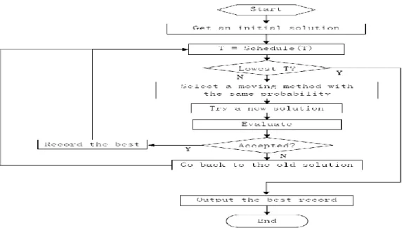
Annealing indicates the process being occurs when the physical substances, for example metal, were raised and get a high energy level after that gradually cooled down until some solid state level is reach. The objective for process is to achieve the minimum energy state. In this process, physical substances or materials were usually move from higher energy level to lower. If the cooling process is slow certainly, the minimization will be happened. Since the algorithm is a natural process, the natural variability was be concerned. There are some probabilities at each stage for the cooling process could be a chance of transition to a higher energy state will happen.
However, as energy state being naturally decline, the probability that moving to higher energy state will be decreased.
The simulated annealing randomly choose an initial point to start within its search space. From this point, the search space will be predetermined by user. The new optimum point acquired is then compared to the initial point in order to check if the new optimum point is better. For minimization case, if the optimum value is tend to be decreasing, it will be accepted and the algorithm will keep going to search the better optima.
Higher optima value for the objective function may be accepted with a certain probability that will be determined by Metropolis criteria. To accept the points with higher optima values, the algorithm is able to escape the local optima. As the algorithm being processing, the length of the steps became shorter, and the final solutions will be close.
Basically, the Mertropolis criteria using the initial user defined parameters, T which refers to temperature, and RT refers to temperature reduction factor, to precisely determine the probability of accepting the higher optimum value of the relating objective function.
Figure 2.2: Evolution flow of Simulated Annealing (Reference from intechopen.com)
2.1.3 Evolutionary Algorithm (EA)
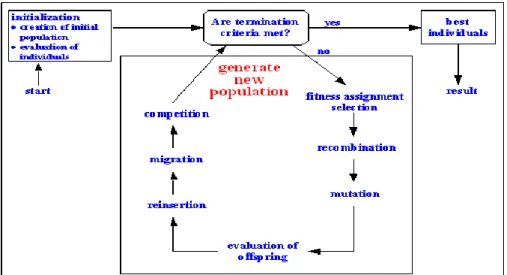
The EA algorithm was suggested to modify to many different variants in various field. However, all these techniques used is the same, it’s given a population size of the individuals with the environmental pressure lead to natural selection, and this can cause a rise in the population size. In order to maximize the quality of related solution, we can create a set of candidate solutions randomly, for example, function’s search space’s domain. From this, the EA algorithm can choose better candidates to seed for next generation by using recombination or/and mutation to them.
Recombination operator applied to at least two candidates (so called parents) and this will results at least one new candidate (children). Mutation operator was applied to a candidate and results a one new candidate. In summation, execution of recombination and mutation results to a new set of candidates. One iteration will having one process of this. The process could be iterated until a candidate with best quality is found or predetermine iteration setting by user is reached. There have two fundamental forces which form the EA basis, there are:
Variation operators that create the diversity.
Selection that will be consider act as force pushing to better quality.
The applications with variations and selection usually lead to an improved optimum solution. It is simple to see whether the EA algorithm is optimising by observed the results whether is approaching optimal values closer and closer.
Figure 2.3: Evolution flow of Evolutionary Algorithm (Reference from http://www.geatbx.com/docu/algindex-01.html)
2.2 Particle Swarm Optimization (PSO)
Particle Swarm Optimization was introduced in 1995 by Kennedy and Eberhart. The first antecedent of this system were in 1983, working by Reeves. He proposed the particle systems to model objects that are dynamic and the objects are very abstract which cannot be known as polygon or surface. Such objects like fire, smoke and clouds. The moving position of each particle is independent, and the direction of movement was governed by the rules. In 1987, Reynolds used the system to simulate the behaviour of bird flocking. In 1990, the Heppner and Grenander included a roost that was attractive to the simulated birds. Set of rules was inspired by these two models and been using on this system nowadays.
Based on the social psychology research, the dynamic theory of social impact, was the another first inspiration to build up the particle’s system. The algorithms and rules governed the direction and movement of the particles in particular search space, it also can be treated as a model of social behaviour.
2.2.1 Swarm Intelligence
Swarm intelligence was widely using on the Particle Swarm Optimization, It also can said to be core of Particle Swarm Optimization. Swarm intelligence is refer to the dealing of naturals and artificials system composed to multiple individuals using decentralized and self-organization. In particular, the collective of the particles depends on locals interaction with each other and also with their environments culture. For such, the particles systems studied by swarm intelligence are bird flocking, nest swarming, fish schooling and herds of land animal. Some human artifacts also behave with swarm intelligence such as some multi-robots system and some programmes were written to simulate some optimization or data analysis.
The swarm intelligence has few properties that made the Particle Swarm Optimization powerful.
1) It is composed of multiple individuals.
2) The individuals are relatively homogenous, they are all similar or identical either they are belongs to a few topologies.
3) Their interactions are based on the simple behavioural rules and only interact with using their local information that they exchange directly.
4) The overall interactions are based on their environmental information and conditions.
The swarm intelligence have no coordinate for the individual to interact each other. Furthermore, each of the individuals interact each other by without any controller. Each individual are self-adjust interactions with their known local information. Many animals interact with each other using the swarm intelligence, such as when the bird is flocking, the birds interacts with each other without any collision and crossing to each other due to the self-controlled within their search space.
Due to the properties of swarm intelligence in above, it is possible to design swarm intelligence with characteristics of scalable, parallel and fault tolerant.
2.3 Unique PSO
Kennedy and Eberhart introduced optimization of mathematical function by PSO. Assume there is an n-dimensional multivariable function to be optimized. The function may be represented as,
where is vector of search space variable, which represents the vector of the variables of the given function. This could be help to find out the function’s local optimum is whether minimum or maximum point.
Example: Simple two-dimensional sphere function was considered and the equation given as below,
It is obviously to show that the optimum point is minimum (0,0) to get = 0. It’s even does not require to use handwritten calculation due to its single global optimum.
It’s tough to optimize multivariable function with multi-peaks. For such function as below,
For such function, there have peaks and a rough fitness lands. The function was plotted in Figure 2.4. It is complicate to optimize the function using handwritten calculation and its take a long time to finish. To search for the function’s global optimum, Kennedy and Eberhart adapting the PSO method into the function. The system’s particles swarm over the rough lands of function with their own information.
So every peaks of the function could be swarmed by the particles. It’s called multi- agent parallel search technique. Every particle has its own velocity and position. And they do sharing about their information to each other. Hence, they could swarm in more effectively and efficiently.
Figure 2.4: Multi-peaks function as mentioned as above. (Copyright Swagatam Das)
2.4 PSO Algorithm Flowchart
Yes No
Yes No
Initialize particles
Calculate each fitness value for particles
Is it the current value better than Pbest?
Assign the value to Pbest
Keep previous Pbest as current
Pbest
Assign Pbest to Gbest
Calculate velocity for each particle
Use each particle’s velocity value to calculate the own value
Maximum epochs reached?
End
CHAPTER 3
3 METHODOLOGY
The optimization problems were concerned on some mathematical functions and mechanical/mechatronics components with subject to nonlinear constraints equations. The problem’s methodology consists of the designed equation and fitness function which required to be optimized by the PSO method. Some designed parameters for PSO were introduced on the following topics, for such parameters are iterations, population size and others PSO variables parameters.
3.1 Optimization of Rosenbrock function
This function also known as banana function, due to its shape looks like banana shape and have a pattern of non-convex. The global minimum is inside a long, narrow and shape parabolic. It basically have two variables which are and . The function’s equation is described as follows,
(3.1)
where a and b are 1 and 100 respectively. The global minimum point is (1,1), and will results to 0 of . The shape of the function simulated as follows,
Figure 3.1: Rosenbrock function
3.2 Optimization of Matyas function
The Matyas function have a shape same as the rosenbrock function. However, the global minimum is different. The function defined as,
(3.2)
The global minimum point is (0,0), and will results to 0 of . The shape of the function simulated as follows,
Figure 3.2: Matyas function
3.3 Weight Minimization of Speed Reducer(WMSR)
The objective of the problem is minimization of speed reducer weight.
Effectively, it could maintain the maximum efficiency of rotational speed of two shafts. The speed reducer structure contains of a gear, pinion and two shafts. There are one fitness function, and 11 constraints equations with 7 design variables.
Figure 3.3: Speed reducer design actual diagram
Figure 3.4: Speed reducer design structure diagram
Shaft 1 Shaft 2
Gear 1
Gear 2
Bearing 1 Bearing 2
The design variables required to be optimized are the width of the face (b = ), the teeth model (m = ), number of teeth on the pinion (n = ), length of the shaft 1 between the bearings ( = ), length of the shaft 2 between the bearings ( ), shaft 1 diameter ( ), shaft 2 diameter ( ). The fitness function and its constraints formulae were given as follows,
(3.3.1)
Subject to
The ranges of the design variables were used as follows,
3.4 Weight Cost Minimization of Pressure Vessel (WMPL)
The objective of the problem is to minimize total weight of the pressure vessel. Vessel with shape of cylindrical is capped at both ends with hemispherical heads as shown figure 1.
Figure 3.5: Pressure vessel design actual diagram (Reference from libertyengg.com)
Figure 3.6: Pressure vessel design structure diagram
Weight that need to be minimized including cost material, forming and the welding. There are four design variables which are thickness of the shell ( ), thickness of the head ( ), radius of the inner part of the cylinder tube ( ), length of the part of the cylindrical tube ( ). and are integers multiplies of 0.0625 inch, which made the thicknesses of rolled steel plates available. and are continuous values. The fitness function and its constraints formulae were given as follows,
Subject to
The ranges of the design variables were used as follows,
3.5 Volume Minimization of Compression Spring (VMCS)
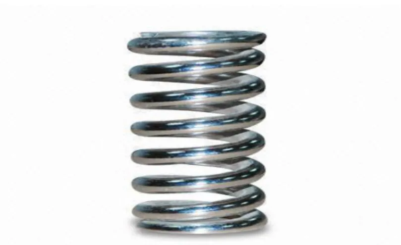
The objective is to minimize the volume of the compression spring. The structure of the spring was shown as figure 1.
Figure 3.7: Tension/Compression Spring actual diagram (Reference from globalsources.com)
Figure 3.8: Tension/Compression Spring structure diagram Free Length
Displacement
There are three design variables which are the number of active coils of the spring ( ), the winding diameter ( ), the wire diameter ( ). The fitness function and its constraints formulae were given as follows,
Subject to
The ranges of the design variables were used as follows,
3.6 Particle Swarm Optimization (PSO) Algorithm
There have two algorithms were used to optimize the above mechanical components problems, which are Basic PSO and Accelerated PSO. Accelerated PSO algorithm is a modified version of Basic PSO, it were used to improve the speed of convergence, which could save a lot time. In this paper, BPSO and APSO were implemented on the above optimization problems, and comparison for these both results was worked out.
3.6.1 Basic Particle Swarm Optimization (BPSO)
BPSO is original algorithm which proposed by Kennedy and Eberhart.
Furthermore, it is a population based evolutionary algorithm. Development of the algorithm was inspired by the social nature behavior such as bird flocking. It simulates a group of individuals called particles in a problem’s search space. The particles swarm over the search space to find the optimal solution. The way of swarming was fixed by the velocity update equations and be described as follows,
where and is self-confidence factor and swarm-confidence factor respectively.
and required to be set for ensuring better coverage of the design space and reduce the possibility of entrapment in local optima. The is the velocity of particle at time . The is the velocity of particle at time . The is the best position of each particle over time. The is the best global solution in the current swarm. The is the best fitness location has been achieved so far. Previous research papers were using the values of 2 and 2 for and respectively to get best optimum solutions. In this paper, in order to improve the convergence rate, reduced and factors values to an acceptable range of 0-1 were implemented by reducing the randomness of the particles as iterations proceed. The algorithm can be described by monotonically decreasing function as follows,
or
where is the initial value of randomness parameter which in the range of 0.5~1.
The is number of iterations or the time steps. is a control parameter. In this paper, and were used to implement reduction of randomness.
Hence, the equation can be concluded as,
where is the maximum iterations.
3.6.2 Accelerated PSO (APSO)
The basic particle swarm optimization uses both global best, and individual best, to determine optimal solution of the related problems. The reason of using the individual best, is for the purpose of increasing the diversity in the quality of the solutions. However, this diversity can be simulated using some randomness. There is no compelling reason to use the individual best, unless the optimization problem is highly non-linear and multimodal.
In order to accelerate the convergence speed, APSO algorithm were developed by using the global best only. Reduction of randomness also was implemented in this algorithm to improve the convergence. The algorithm equation is described as follows,
where is drawn from random numbers in range of 0~1. The position update equation is just simply as follows,
Reduction of randomness also was implemented in this algorithm to improve the convergence. The decreasing function’s parameters were same as the BPSO algorithm mentioned.
CHAPTER 4
4 RESULTS AND DISCUSSIONS
In this chapter, simulation results for the optimization problems which mentioned above were recorded. The recorded results included some concerned parameters, such as iterations, population size, and also fixed value for self- confidence factor and swarm-confidence factor. Those parameters could hugely affect the simulation results. Moreover, the comparisons of the BPSO and APSO were discussed in this chapter for each of the problems. The recommended PSO parameters for each problems were also concluded in this paper.
4.1 Optimization of Rosenbrock function
The results for this problem is including three variables that needed to be optimized, which are and . Following tables give the numerical results using population size of 20, 40, 60, 80 and 100.
Table 4.1: Comparison results and between BPSO and APSO algorithms, n= 20 (Rosenbrock).
Global best, Global best, Global best, fmin
BPSO APSO BPSO APSO BPSO APSO
20 200 0.9952 0.9969 0.9904 0.9926 0.0000 0.0001 Elapsed time, (seconds) 0.004236 0.002589
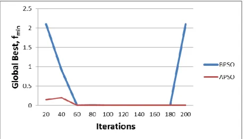
Figure 4.1: Convergence graph of global optimum, fmin by BPSO and APSO using population size of 20 over 200 iterations.
Table 4.2: Comparison results and between BPSO and APSO algorithms, n=40 (Rosenbrock).
Global best, Global best, Global best, fmin
BPSO APSO BPSO APSO BPSO APSO
40 180 1.0044 1.0004 1.0088 1.0008 0.0000 0.0000 Elapsed time, (seconds) 0.002396 0.001935
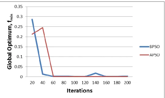
Figure 4.2: Figure 4.1.2: Convergence graph of global optimum, fmin by BPSO and APSO using population size of 40 over 200 iterations (Rosenbrock).
Table 4.3: Comparison results and between BPSO and APSO algorithms, n=60 (Rosenbrock).
Global best, Global best, Global best, fmin
BPSO APSO BPSO APSO BPSO APSO
60 200 1.0000 0.9999 0.9999 0.9998 0.0000 0.0000 Elapsed time, (seconds) 0.003558 0.003987
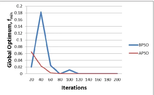
Figure 4.3: Convergence graph of global optimum, fmin by BPSO and APSO using population size of 60 over 200 iterations (Rosenbrock).
Table 4.4: Comparison results and between BPSO and APSO algorithms, n=80 (Rosenbrock).
Global best, Global best, Global best, fmin
BPSO APSO BPSO APSO BPSO APSO
80 200 1.0000 1.0000 1.0000 1.0000 0.0000 0.0000 Elapsed time, (seconds) 0.002821 0.001651
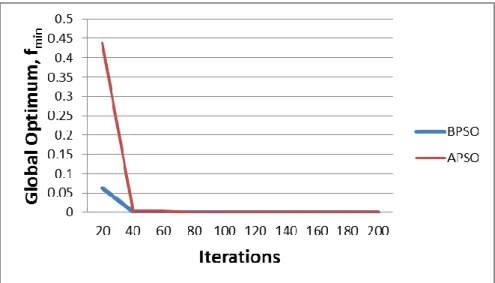
Figure 4.4:Convergence graph of global optimum, fmin by BPSO and APSO using population size of 80 over 200 iterations (Rosenbrock).
Table 4.5:Comparison results and between BPSO and APSO algorithms, n=100 (Rosenbrock).
Global best, Global best, Global best, fmin
BPSO APSO BPSO APSO BPSO APSO
100 200 1.0000 1.0000 1.0000 1.0000 0.0000 0.0000 Elapsed time, (seconds) 0.002973 0.002301
Figure 4.5: Convergence graph of global optimum, fmin by BPSO and APSO using population size of 100 over 200 iterations (Rosenbrock).
Figure 4.6:Elapsed time by simulation of BPSO and APSO against population size (Rosenbrock).
Table 4.6:Accuracy results of x and y between BPSO and APSO algorithms (Rosenbrock).
Exact value, fmin Overall global best, fmin
BPSO APSO
0.0000 0.0000 0.0000
Accuracy (%) 99.9999 99.9999
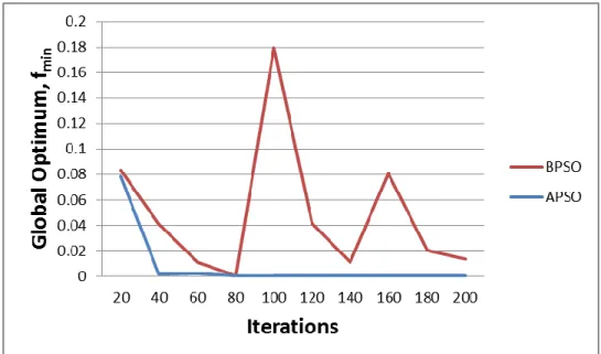
Overall view of the results show the global optimum, fmin were fast reach over 200 iterations when the population size was increasing, since the population size refers to the number of particles that responsible to swarm over the problem’s search space to the optimum point. Figure 4.1 shows the global optimum’s convergence using APSO algorithm is faster reach to convergence point compared to BPSO algorithm as it using the population size of 20. As the population size increasing, the acceleration for convergence using BPSO exceeded the acceleration using APSO.
Figure 4.5 shows the BPSO algorithm was converging to the global optimum faster than APSO algorithm. Using 20, 40, 60, and 80 of population size was yield for fluctuation results for BPSO. This unstable situation can be explained by the BPSO algorithm is using both current global best, and individual best, that need use more particles than APSO which just using global best, to find the optimum point.
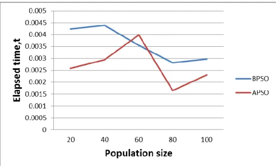
From the Figure 4.1.6, the elapsed time for BPSO was about fluctuated within 0.0025-0.0045 seconds over 100 population size. And the elapsed time for APSO was about fluctuated within 0.0015 – 0.0040 seconds over population size. These small changes of time for both algorithms may due to the low complexity of the fitness function.
4.2 Optimization of Matyas function
The results for this problem also including three variables that needed to be optimized, which are and . Theoretically, the results give 0, 0, and 0
and respectively. Following tables give the numerical results using population size of 20 and population size of 40.
Table 4.7:Comparison results and between BPSO and APSO algorithms, n=20 (Matyas).
Global best, Global best, Global best, fmin
BPSO APSO BPSO APSO BPSO APSO
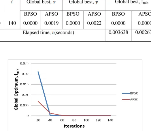
20 140 0.0000 0.0019 0.0000 0.0022 0.0000 0.0000 Elapsed time, (seconds) 0.003638 0.002635
Figure 4.7:Convergence graph of global optimum, fmin by BPSO and APSO using population size of 20 over 140 iterations (Matyas).
Table 4.8: Comparison results and between BPSO and APSO algorithms, n=40 (Matyas).
Global best, Global best, Global best, fmin
BPSO APSO BPSO APSO BPSO APSO
40 140 0.0000 0.0000 0.0000 0.0000 0.0000 0.0000 Elapsed time, (seconds) 0.002989 0.002930
Figure 4.8:Convergence graph of global optimum, fmin by BPSO and APSO using population size of 40 over 140 iterations (Matyas).
Figure 4.9:Elapsed time by simulation of BPSO and APSO against population size (Matyas).
Table 4.9:Accuracy results and between BPSO and APSO algorithms (Matyas).
Exact value, fmin Overall global best, fmin
BPSO APSO
0.0000 0.0000 0.0000
Accuracy (%) 99.9999 99.9999
In this optimization, the BPSO gives the results for faster converge to the optimum point compared to APSO results even using 20 and 40 of population size.
In figure 4.6, the exact value of optimum point, 0 was reached at iteration of 40th by using BPSO, which is faster convergence compared to APSO which reach optimum point at iterations of 60th. In figure 4.7, BPSO converge to optimum point at 20th of iterations and remain constant to the end of the iterations, while the APSO results a converging point at 40th of iterations. This can be concluded that, in this case problem, BPSO algorithm gives better convergence speed since it needed less population size to optimize even 20. The elapsed time for BPSO was about fluctuated within 0.0029-0.0037 seconds over 100 population size. And the elapsed time for APSO was about fluctuated within 0.0025 – 0.0030 seconds over 100 population size.
4.3 Weight Minimization of Speed Reducer (WMSR)
The results for this problem is including 7 variables that needed to be optimized, which are the width of the face (b = 𝑥1), the teeth model (m = 𝑥2), number of teeth on the pinion (n = 𝑥3), length of the shaft 1 between the bearings (𝑙1 = 𝑥4), length of the shaft 2 between the bearings (𝑙2 =𝑥5), shaft 1 diameter (𝑑1=𝑥6), shaft 2 diameter (𝑑2=𝑥7) and .
Table 4.10:Comparison overall global best between BPSO and APSO algorithms with population, n =20 (WMSR).
n Global best BPSO APSO
20 160 ( ) 3.5000 3.5000
( ) 0.7000 0.7000
( ) 17.0000 17.0011
( ) 7.3000 7.9903
( ) 7.8000 7.8053
( ) 3.3502 3.3516
( ) 5.2867 5.2869
( ) 2996.3000 3003.1000
Figure 4.10:Convergence graph of global optimum, fmin by BPSO and APSO using population size of 20 over 160 iterations (WMSR).
Table 4.11:Comparison overall global best between BPSO and APSO algorithms with population, n =40 (WMSR).
Figure 4.11:Convergence graph of global optimum, fmin by BPSO and APSO using population size of 40 over 160 iterations (WMSR).
n Global best BPSO APSO
40 160 ( ) 3.5000 3.5001
( ) 0.7000 0.7000
( ) 17.0000 17.0000
( ) 7.3000 7.8000
( ) 7.8000 7.3058
( ) 3.3502 3.3504
( ) 5.2867 5.2869
( ) 2996.4000 3000.2000
Table 4.12:Comparison overall global best between BPSO and APSO algorithm with population, n =60 (WMSR).
Figure 4.12:Convergence graph of global optimum, fmin by BPSO and APSO using population size of 60 over 160 iterations (WMSR).
n Global best BPSO APSO
60 160 ( ) 3.5004 3.5001
( ) 0.7000 0.7000
( ) 17.0000 17.0000
( ) 7.3062 7.8002
( ) 7.8002 7.3798
( ) 3.3504 3.3504
( ) 5.2867 5.2868
( ) 2996.7000 3004.0000
Table 4.13:Comparison overall global best between BPSO and APSO algorithm with population, n =80 (WMSR).
Figure 4.13;Convergence graph of global optimum, fmin by BPSO and APSO using population size of 80 over 160 iterations (WMSR).
n Global best BPSO APSO
80 160 ( ) 3.5000 3.5001
( ) 0.7004 0.7000
( ) 17.0000 17.0000
( ) 7.3006 7.8000
( ) 7.8000 8.1543
( ) 3.3503 3.3520
( ) 5.2867 5.2867
( ) 2996.4000 3000.1000
Table 4.14:Comparison overall global best between BPSO and APSO algorithm with population, n =100 (WMSR).
Figure 4.14:Convergence graph of global optimum, fmin by BPSO and APSO using population size of 100 over 160 iterations (WMSR).
n Global best BPSO APSO
100 160 ( ) 3.5000 3.5000
( ) 0.7004 0.7000
( ) 17.0000 17.0000
( ) 7.3001 7.6242
( ) 7.8000 7.9011
( ) 3.3502 3.3509
( ) 5.2867 5.2868
( ) 2996.4000 3001.7000
Figure 4.15:Elapsed time by simulation of BPSO and APSO against population size (WMSR).
Table 4.15:Comparison overall best solutions(WMSR) by BPSO, APSO,EA-Coello (WMSR).
Overall best solution BPSO APSO EA-Coello
( ) 3.5000 3.5001 3.506163
( ) 0.7004 0.7000 0.700831
( ) 17.0000 17.0000 17.0000
( ) 7.3006 7.8000 7.460181
( ) 7.8000 8.1543 7.9632
( ) 3.3503 3.3520 3.3629
( ) 5.2867 5.2867 5.3089
( ) 2996.4000 3000.1000 3.025.0051
From the results shown, the weight needed to be minimized is around 3000kg.
Both algorithms were used to perform the optimization and both gives global optimum at around 3000kg. However, the global optimum obtained by BPSO is slightly lower than the global optimum obtained by APSO, which the best global optimum obtained is 2996.4000kg for BPSO and 3001.7000kg for APSO. BPSO has increasing its convergence speed as the population size was increasing and also its convergence becoming stable over iterations. From the Figure 4.3.6, the elapsed time for BPSO and APSO over population size is almost the same. Both algorithm elapsed times rapidly increasing from population size of 60 to 100.
4.4 Weight Minimization of Pressure Vessel (WMPV)
The results for this problem is including the thickness of the shell ( ), thickness of the head ( ), radius of the inner part of the cylinder tube ( ), length of the part of cylindrical tube ( ) and . Table 4.4.1-4.4.10 gives results using population size of 20, 40, 60, 80 and 100 by two algorithms BPSO and APSO.
Below figures give line graph of global minimum, over 160 iterations.
Table 4.16:Comparison overall global best between BPSO and APSO algorithm with population, n =20 (WMSR).
n Global best BPSO APSO
20 200 ( ) 0.8111 0.8087
( 0.4013 0.3993
( ) 42.0116 41.2638 ( ) 177.7085 177.8766
( ) 5946.4000 6103.7000
Figure 4.16:Convergence graph of global optimum, fmin by BPSO and APSO using population size of 20 over 200 iterations (WMSR).
Table 4.17:Comparison overall global best between BPSO and APSO algorithm with population, n =40 (WMSR).
n Global best BPSO APSO
40 200 ( ) 0.7781 0.7827
( 0.3846 0.3869
( ) 40.3173 40.5450 ( ) 200.0000 197.1924
( ) 5884.5000 5900.7000
Figure 4.17:Convergence graph of global optimum, fmin by BPSO and APSO using population size of 40 over 200 iterations (WMSR).
Table 4.18:Comparison overall global best between BPSO and APSO algorithm with population, n =60 (WMSR).
n Global best BPSO APSO
60 200 ( ) 0.7781 0.7938
( 0.3846 0.3942
( ) 40.3173 41.1259 ( ) 200.0000 189.4270
( ) 5884.6000 5926.3000
Figure 4.18:Convergence graph of global optimum, fmin by BPSO and APSO using population size of 60 over 200 iterations (WMSR).
Table 4.19:Comparison overall global best between BPSO and APSO algorithm with population, n =80 (WMSR).
n Global best BPSO APSO
80 200 ( ) 0.8028 0.8140
( 0.3968 0.4025
( ) 41.5966 42.1728 ( ) 182.9249 175.7244 ( ) 5928.1000 5950.3000
Figure 4.19:Convergence graph of global optimum, fmin by BPSO and APSO using population size of 80 over 200 iterations (WMSR).
Table 4.20:Comparison overall global best between BPSO and APSO algorithm with population, n =100 (WMSR).
n Global best BPSO APSO
100 200 ( ) 0.7781 0.7872
( 0.3846 0.3902
( ) 40.3173 40.7853 ( ) 200.0000 193.6048
( ) 5884.5000 5904.0000
Figure 4.20:Convergence graph of global optimum, fmin by BPSO and APSO using population size of 100 over 200 iterations (WMSR).
Figure 4.21:Elapsed time by simulation of BPSO and APSO against population size (WMSR).
Table 4.21:Comparison overall best solutions by BPSO, APSO and EA-Coello algorithm (WMSR).
From the results shown, the weight needed to be minimized is around 6000kg.
Both algorithms were used to perform the optimization and both gives global optimum at around 6000kg. However, the global optimum obtained by BPSO is slightly lower than the global optimum obtained by APSO, which the best global optimum obtained is 5884.5000kg for BPSO and 5904.0000kg for APSO. BPSO has increasing its convergence speed as the population size was increasing and also its convergence becoming stable over iterations. In this problem optimization, the convergence using APSO has much more higher acceleration than the BPSO, particularly when increasing the population size. As the population size was set to 100, the convergence to the optimal point using APSO was started at almost at around 20th iterations. On the other side, the convergence using BPSO was started at lately around 100th iterations. This may due to the settings of the various lower and upper boundaries for every type of the problems. From the Figure 4.4.6, the elapsed time for BPSO and APSO over population size is almost the same. The time increasing time over the population size for both algorithms are almost the same.
Overall best solution BPSO APSO EA-Coello
( ) 0.7781 0.7872 0.8125
( 0.3846 0.3902 0.4375
( ) 40.3173 40.7853 40.3239
( ) 200.0000 193.6048 200.0000 ( ) 5884.5000 5904.0000 6288.7445
4.5 Volume Minimization of Compression Spring (VMCS)
The results for this problem is including 3 variables and one global best, that were been optimized, which are the number of active coils of the spring ( ), the winding diameter ( ), the wire diameter ( ) and the volume need to be optimized, . Table 4.5.1-4.5.10 gives the numerical results using population size of 20, 40, 60, 80 and 100 by two algorithms BPSO and APSO. Below figures give line graph of global minimum, over 200 iterations.
Table 4.22:Comparison overall global best between BPSO and APSO algorithm with population, n =20 (VMCS).
Figure 4.22:Convergence graph of global optimum, fmin by BPSO and APSO using population size of 20 over 200 iterations (VMCS).
n Global best BPSO APSO 20 200 (Ts) 0.0526 0.0500 (Tb) 0.3792 0.3174 (Ts) 10.0854 14.0301
( ) 0.0127 0.0127
Table 4.23;Comparison overall global best between BPSO and APSO algorithm with population, n =40 (VMCS).
Figure 4.23:Convergence graph of global optimum, fmin by BPSO and APSO using population size of 40 over 200 iterations (VMCS).
n Global best BPSO APSO 40 200 (Ts) 0.0501 0.0500 (Tb) 0.3191 0.3174 (Ts) 13.8917 14.0358
( ) 0.0127 0.0127
Table 4.24:Comparison overall global best between BPSO and APSO algorithm with population, n =6 (VMCS).
Figure 4.24:Convergence graph of global optimum, fmin by BPSO and APSO using population size of 60 over 200 iterations (VMCS).
n Global best BPSO APSO 60 200 (Ts) 0.0500 0.0500 (Tb) 0.3174 0.3174 (Ts) 14.0278 14.0281
( ) 0.0127 0.0127
Table 4.25:Comparison overall global best between BPSO and APSO algorithm with population, n =80 (VMCS).
Figure 4.25:Convergence graph of global optimum, fmin by BPSO and APSO (VMCS).
n Global best BPSO APSO 80 200 (Ts) 0.0500 0.0522 (Tb) 0.3174 0.3684 (Ts) 14.0278 10.6366
( ) 0.0127 0.0127
Figure 4.26:Elapsed time by simulation of BPSO and APSO against population size (VMCS).
Table 4.26:Comparison overall best solutions by BPSO, APSO and Coello algorithm (VMCS).
Both algorithms were used to perform the optimization and both gives global optimum at around 0.013kg. Both algorithms have the best optimum point of 0.0127kg. BPSO has increasing its convergence speed as the population size was increasing and also its convergence becoming stable over iterations. In this problem optimization, Most of the simulations give the convergence of range in 0.0127 to 0.02 for population size 20, 40, 60, and 80. At population size of 20, there is a larger fluctuation of the optimum point at between 160th and 200th iterations, this may due to the insufficient of the population size needed to be swarm over the optimum point.
Overall best solution BPSO APSO Coello
(Ts) 0.0500 0.0522 0.0514
(Tb) 0.3174 0.3684 0.3516
(Ts) 14.0278 10.6366 11.6322
( ) 0.0127 0.0127 0.0127
From the Figure 4.5.5, the trend of time increasing time over the population size is almost the same as the previous pressure vessel’s optimization result. Overview of all these results, it can be concluded that, the optimization problem consists of multiple constraints needed more time to be optimized particularly the population was set is larger.
CHAPTER 5
5 CONCLUSION AND RECOMMENDATIONS
5.1 Conclusions
According to results, all related problems were optimized successfully, and some recommendations were introduced at below. From the results simulated, mathematical function (Rosenbrock and Matyas function) require lesser population size to achieve their optimum point compared to the mechanical optimization problems (WMSR, WMPV,VMCS). This may due to the dependence of simplicity of the functions, which the WMSR, WMPV and VMCS problems involving the inequalities constraints.
Due to the exist only one objective function of Rosenbrock and Matyas, the complication for the optimization also tend to decrease, this lead to a short time elapsed for optimization. The elapsed times for both mathematical functions are quite stable when the population size was increasing, and was not exceed 0.005 seconds.
Compared to WMSR, WMPV and VMCS, due to its problem including a lot of inequalities constraints, the time elapsed was increasing over the population size. As we can complexity of the design problems was higher, the time elapsed for optimization will be longer. Such as the WMSR, there have one objective function and 11 inequalities constraints, the time elapsed also the highest among these three mechanical optimization problems which the time taken at around 4.4 seconds.
For the optimization of the Rosenbrock and Matyas function, the APSO acceleration was not stable, meant sometimes it accelerating slower than BPSO over the population size. This may due to the complexity of the mathematical function are extremely low, so the population size used for BPSO can be as low as APSO to
achieve convergence in same time or even faster than APSO. For the mechanical optimization, due to the high complexity with subject to constraints, the BPSO require more particles solution (population size) to converge to the optimal solutions.
On the other hand, WMSR and WMPV optimized by APSO algorithm were successfully accelerated compared to BPSO, since the APSO only using the global best, , therefore the population size could be decreased. In summation, the APSO using less population size then BPSO to converge to optimal solutions, this could save some elapsed time. However, for VMCS problem, both algorithm were converge in same acceleration, this may due to the search space set by the boundaries were small enough to converge at the beginning of the convergence, therefore both algorithms were not limited by the population size.
5.2 Recommendations
The optimization method is tend be subjective. The setting parameters for PSO method would depend on what target that user want to achieve. The modified algorithm was not achieved better result at all the concerned problems. Therefore, there are several recommendations for the setting parameters for each optimization problems. The best setting parameters was chose which depend on the convergence stability which led by population size and iterations.
5.2.1 Rosenbrock functions
APSO is recommended to this function since APSO gives a more stable convergence than BPSO even in low population size. The population size and iterations recommended for this is 80 and 140 respectively.
5.2.2 Matyas function
APSO is recommended to this function since APSO gives a more stable convergence than BPSO even in low population size. The population size and iterations recommended for this is 50 and 140 respectively.
5.2.3 Weight Minimization of Speed Reducer (WMSR)
BPSO is recommended for this optimization problem since it gives best optimal solution compared to APSO and EA-Coello. The population size and iterations recommended for this is 80 and 120 respectively.
5.2.4 Weight Minimization of Pressure Vessel (WMPV)
BPSO is recommended for this optimization problem since it gives best optimal solution compared to APSO and EA-Coello. The population size and iterations recommended for this is 100 and 120 respectively.
5.2.5 Volume Minimization of Compression Spring (VMCS)
In this problems both algorithm gives same results and the stability of the convergence are almost the same. Therefore, both algorithm is recommended to this problem The population size and iterations recommended for this is 100 and 100 respectively.
REFERENCES
Afonso C.C. Lemongea, H. J. B. C. C. B. a. F. B., 2010. Constrained optimization problems in mechanical engineering design using a real-coded steady-state genetic algorithm.
al., m. D. e., 2008. Particle Swarm Optimization. Particle Swarm Optimization, Volume 1486, p. 3(11).
Bakshi, A. P. P. a. G. J., n.d. Pullulanase and alpha-amylase production by a Bacillus cereus isolate. Issue Letter in Applied Microbiology, pp. 210-213.
Birattari, M. D. a. M., 2007. Swarm inteliigence. Swarm Intelliigence, Volume 1462, p. 2(9).
Cohanim, R. H. a. B., n.d. A comparison of Particle Swarm optimization and Genetic Algorithm.
Ketan Tambolia*, S. P. P. R. S., 2014. Optimal Design of a Heavy Duty Helical Gear Pair using Particle. 2nd International Conference on Innovations in Automation and Mechatronics Engineering,, pp. 513-519.
Report, M. E. H. P. H. L. T., 201. Good parameters for Particle swarm optimization.
Rossana M. S. Cruz1, H. M. P. a. R. M. M., n.d. Artificial Neural Networks and Efficient Optimization Techniques for Applications in Engineering.
Sexton, R. S., n.d. Optimization of Neural Networks: A Comparative Analysis of the Genetic Algorithm and Simulated Annealing.
Swagatam das, A. A. a. A. K., n.d. Particle Swarm optimization and Differential Evolution Algorithm. Technicall Analysis, Applications and Hybridisation Perspectives.
Xiaobui Hu, R. C. E. Y. S., n.d. Engineering optimization with Particle Swarm.
Yangyang Li, L. J. R. S. R. S., 2015. Dynamic-context cooperative quantum-behaved particle swarm optimization based on multilevel thresholding applied to medical image segmentation. pp. 408-422.
APPENDICES
APPENDIX A: MATLAB codes(BPSO)
% Optimization of speed reducer using Basic PSO function bpso
tic
%% Lower and upper bounds
Lb=[2.6 0.7 17 7.3 7.8 2.9 5];
Ub=[3.6 0.8 28 8.3 8.3 3.9 5.5];
% Default parameters [number of particles, number of iterations]
para=[100 160 0.95];
% Call the baic PSO optimizer
[gbest,fmin]=pso_mincon(@cost,@constraint,Lb,Ub,para);
% Display results
Bestsolution=gbest fmin
toc
%% Objective function function f=cost(x)
f=0.7854*x(1)*(x(2)^2)*(3.3333*(x(3)^2)+14.9334*x(3)-43.0934)-
1.508*x(1)*((x(6)^2)+(x(7)^2))+7.4777*(x(6)^3+x(7)^3)+0.7854*(x(4)*(
x(6)^2)+x(5)*(x(7)^2));
% Nonlinear constraints
function [g,geq]=constraint(x)
% Inequality constraints
g(1) = (27/(x(1)*(x(2)^2)*x(3)))-1;
g(2) = (397.5/(x(1)*(x(2)^2)*(x(3)^2)))-1;
g(3) = (1.93*(x(4)^3)/(x(2)*x(3)*(x(6)^4)))-1;
g(4) = (1.93*(x(5)^3)/(x(2)*x(3)*(x(7)^4)))-1;
g(5) = (((((745*x(4))/(x(2)*x(3)))^2 + (16.9*10^6))^0.5)/(0.1*(x(6)^3)))-1100;
g(6) = (((((745*x(5))/(x(2)*x(3)))^2 + (157.5*10^6))^0.5)/(0.1*(x(7)^3)))-850;
g(7) = x(2)*x(3)-40;
g(8) = 5-(x(1)/x(2));
g(9) = (x(1)/x(2))-12;
g(10) = (1.5*x(6) +1.9)/x(4) - 1;
g(11) = (1.1*x(7) +1.9)/x(5) - 1;
% If no equality constraint at all, put geq=[] as follows geq=[];
%% === BPSO Solver starts here ================================
function [gbest,fbest]=pso_mincon(fhandle,fnonlin,Lb,Ub,para) if nargin<=4,
para=[100 150 0.95];
end
% Populazation size, time steps and gamma n=para(1); time=para(2); gamma=para(3);
% ---
%% Scalings
scale=abs(Ub-Lb);
% Validation constraints
if abs(length(Lb)-length(Ub))>0,
disp('Constraints must have equal size');
return end
% ---
% Setting parameters alpha, beta
% Randomness amplitude of roaming particles alpha=[0,1]
% Speed of convergence (0->1)=(slow->fast); % beta=0.5 alpha=0.9; beta=0.9;
% A potential improvement of convergence is to use a variable
% alpha & beta. For example, to use a reduced alpha, we have
% gamma in [0.7, 1];
% ---
%% --- Start Particle Swarm Optimization ---
% generating the initial locations of n particles best=init_pso(n,Lb,Ub);
fbest=1e+100;
% --- Iterations starts --- for t=1:time,
% Find which particle is the global best for i=1:n,
fval=Fun(fhandle,fnonlin,best(i,:));
if fval>fbest, pbest=best(i,:);
%fbest=fval;
end
% Update the best if fval<=fbest,
gbest = best(i,:);
fbest=fval;
end end
% ---
% Randomness reduction alpha=newPara(alpha,gamma);
%beta=newPara2(beta,gamma);
% Move all particles to new locations
best=pso_move(best,gbest,pbest,alpha,beta,Lb,Ub);