PREDICTION OF NATURAL GAS MIXTURES PHASE BEHAVIOUR USING EIGHT EOS FUNCTIONS WITH VAN DER WALL AND WONG
SANDLER MIXING RULES
MUHAMAD LUKMAN BIN MANSHOR
MSc. PETROLEUM ENGINEERING UNIVERSITI TEKNOLOGI PETRONAS
JULY 2013
ii
PREDICTION OF NATURAL GAS MIXTURES PHASE BEHAVIOUR USING EIGHT EOS FUNCTIONS WITH VAN DER WALL AND WONG
SANDLER MIXING RULES
By
MUHAMAD LUKMAN BIN MANSHOR
Submitted in partial fulfilment of the requirement of the Master of Science
(Petroleum Engineering)
JULY 2013
Universiti Teknologi PETRONAS Bandar Seri Iskandar
31750 Tronoh
Perak Darul Ridzuan
iii
CERTIFICATION OF APPROVAL
Prediction of Natural Gas Mixtures Phase Envelope using Eight EOS Functions with Van der Wall and Wong Sandler Mixing Rules
by
Muhamad Lukman Bin Manshor
A Project Dissertation submitted to the Petroleum Engineering Programme
Universiti Teknolgi PETRONAS In partial fulfilment of the requirement for the
MSc. PETROLEUM ENGINEERING
Approved by
___________________________
(Dr Khalik M Sabil)
UNIVERSITI TEKNOLOGI PETRONAS TRONOH, PERAK
July 2013
iv
CERTIFICATION OF ORIGINALITY
This is to certify that I am responsible for the work submitted in this project, that the original work is my own except as specified in the reference and acknowledgements, and that the original work contained herein have not been undertaken or done by unspecified sources or persons.
____________________________________________
MUHAMAD LUKMAN BIN MANSHOR
v
ABSTRACT
Prediction of natural gas phase behaviour is important and crucial in hydrocarbon processing industries. This paper main objective is to predict phase envelope of natural gas mixtures by using eight equations of state functions and hence to look at its applicability by comparing the predictions of temperature and pressure from the experimental values conducted for 24 set of natural gas mixtures that comprise of lean natural gases or synthetic natural gases. Hence, the studies of Van der Wall (VDW) and Wong Sandler (WS) mixing rules used with EOS functions are discussed in terms of its significant and validity of the equations to the calculated results. The resulted calculation values of T and P was calculated by using Prode add in Microsoft Excel simulator. For a conclusion, it is found that Soave-Redlich- Kwong (SRK) families with VDW mixing rules have wide applications and are superb in predicting phase behaviours of different mixtures with 83% dominant level compared to Peng-Robinson (PR) families with WS mixing rules when tested for 24 set of natural gas mixtures data. PR-WS is superb at predicting phase behaviours of natural gas mixtures with 25.91% carbon dioxide content, 1.56% of nitrogen and 0.11% of n-hexane. Hence, PR-VDW is superior at predicting synthetic natural gas mixture with 0.77% nitrogen, 1.75% of carbon dioxide, 84.45% of methane, and 0.05% of n-hexane. Thus, the application of PR families is limited for several mixtures only and requires some modification of the EOS parameters. For the effect of different mixing rules used in this study, VDW mixing rules is best described the phase envelopes of natural gas mixtures with different heavies content as heavy as n- octane and its dominated 24 set of mixtures as high as 95% over WS mixing rule.
Therefore, it is conclusive that no single EOS provides reliable predictions of bubble point line and dew point line of all 24 set of natural gas mixtures used in this study and application of VDW mixing rules is reasonable over WS mixing rules, and it is recommended that RK families with Soave temperature functions have wider applications over PR families for this 24 set of natural gas mixtures.
vi
ACKNOWLEDGEMENT
Foremost, I thank God for giving me the opportunity to work on this project. With this gracious I manage to complete this project and thesis. Honestly, the writing of this thesis has been the most challenging part of my academic year.
I would like to acknowledge my supervisor, Dr Khalik M. Sabil for his guidance and support. Though he is a busy man, he was able to spend his quality time by sharing brilliant ideas through my works.
I am especially indebted to my parents and my wife for their patience, support and being a constant source of inspiration during this period.
My thanks to all my friends who have sharing their knowledge and contributing idea throughout this study. Above all I thank to my family and friends who stood beside me and encourage me constantly until the completion of this project.
vii
TABLE OF CONTENTS
ABSTRACT ... v
ACKNOWLEDGEMENT ... vi
TABLE OF CONTENTS ... vii
CHAPTER 1 ... 1
INTRODUCTION ... 1
1.1: An Overview ... 1
1.2: Background of Study ... 3
1.3: Objectives... 3
1.4: Scope of Study ... 4
CHAPTER 2 ... 5
LITERATURE REVIEW... 5
2.1: Introduction ... 5
2.2 Natural Gas... 5
2.3 Applications of the EOS in the Industry ... 8
2.4: About PRODE software in Microsoft Excel Simulation ... 19
CHAPTER 3 ... 21
METHODOLOGY ... 21
3. 1: Introduction ... 21
3. 2: Procedure ... 21
3.3: Procedure Summary ... 23
CHAPTER 4 ... 24
RESULTS AND DISCUSSIONS ... 24
4.1: Introduction ... 24
4.2: Resulted Calculation for SET 6 ... 39
4.2: Resulted Calculation for SET 9 ... 46
4.4: Resulted Calculation for SET 15 ... 49
4.5: Resulted Calculation for SET 18 ... 61
4.6: Resulted Calculation for SET 19 ... 71
4.7: Resulted Calculation for SET 20 ... 75 4.8: Summary of the Resulted Calculation for All Mixtures Used in This Study . 84
viii
CHAPTER 5 ... 102
CONCLUSIONS AND RECOMMENDATIONS ... 102
5.1: Conclusions ... 102
5.2: Recommendations ... 103
REFERENCES ... 104
APPENDIXES ... 107
APPENDIX A ... 107
APPENDIX B ... 119
APPENDIX C ... 123
APPENDIX D ... 155
APPENDIX E ... 175
APPENDIX F ... 183
ix
LIST OF FIGURES
Figure 2. 1: Five Examples of Improved Cubic EOS from the VDW EOS (Velderama, 2003)... 10 Figure 2. 2: Recommendations on Suitability of Modelling Mixtures by EOS
(Velderama, 2003)... 12 Figure 2.3: Recommendation on General EOS and Mixing Rule for Different Types
of Liquid-Vapor Mixtures (Velderama, 2003) ... 12 Figure 2.4: Selected Mixing Rule and Combining Rules Used In Two-Constant
Cubic EOS (Velderama, 2003) ... 13
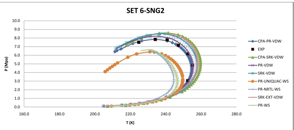
Figure 4. 1: Phase Envelope Generated from Different EOS and Experimental Values for Set 6-SNG 2... 39 Figure 4. 2: Phase Envelope Generated from Different EOSs and Experimental
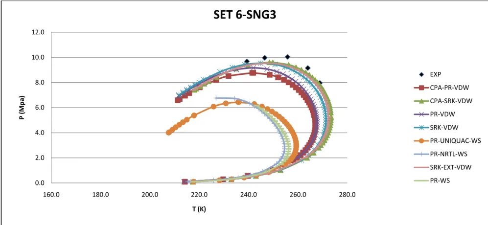
Values for Set 6-SNG... 40 Figure 4. 3: Phase Envelope Generated from Different EOSs and Experimental
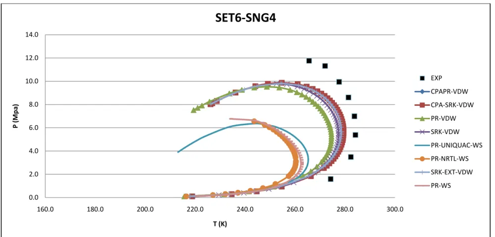
Values for Set 6-SNG 4... 41 Figure 4. 4: Percentage AAD/P Calculated from Different EOSs and Experimental
Values for Set 6 ... 42 Figure 4. 5: Percentage AAD/T Calculated from Different EOSs and Experimental
Values for Set 6 ... 42 Figure 4. 6: Phase Envelope Generated from Different EOSs and Experimental
Values for Set 9-Gas 1 ... 46 Figure 4. 7: Percentage AAD/P Calculated from Different EOSs and Experimental
Values for Set 9 ... 47 Figure 4. 8: Percentage AAD/T Calculated from Different EOSs and Experimental
Values for Set 9 ... 47 Figure 4. 9: Phase Envelope Generated from Different EOSs and Experimental
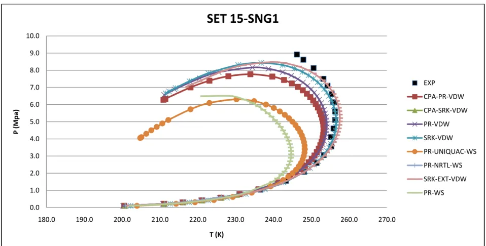
Values for Set 15-Gas 1 ... 49 Figure 4. 10: Phase Envelope Generated from Different EOSs and Experimental
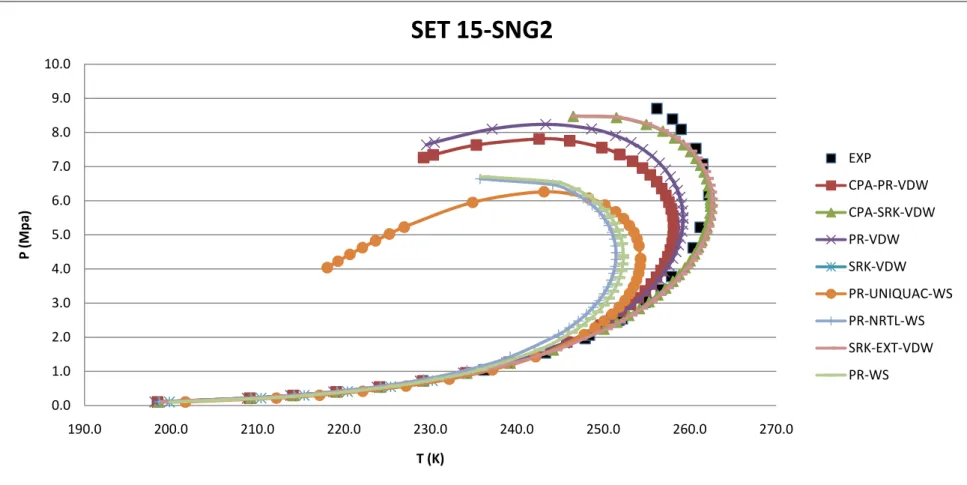
Values for Set 15-Gas 2 ... 50 Figure 4. 11: Phase Envelope Generated from Different EOSs and Experimental
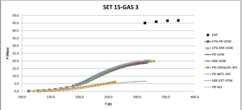
Values for Set 15-Gas 3 ... 51 Figure 4. 12: Phase Envelope Generated from Different EOSs and Experimental
Values for Set 15-SNG 1... 52 Figure 4. 13: Phase Envelope Generated from Different EOSs and Experimental
Values for Set 15-SNG 2... 53 Figure 4. 14: Phase Envelope Generated from Different EOSs and Experimental
Values for Set 15-SNG 3... 54 Figure 4. 15: Phase Envelope Generated from Different EOSs and Experimental
Values for Set 15-SNG 4... 55
x
Figure 4. 16: Phase Envelope Generated from Different EOSs and Experimental Values for Set 15-SNG 5... 56 Figure 4. 17: Percentage AAD/P Calculated from Different EOSs and Experimental
Values for Set 15 ... 57 Figure 4. 18: Percentage AAD/T Calculated from Different EOSs and Experimental
Values for Set 15 ... 58 Figure 4. 19: Phase Envelope Generated from Different EOSs and Experimental
Values for Set 18-SNG 1... 61 Figure 4. 20: Phase Envelope Generated from Different EOSs and Experimental
Values for Set 18-SNG 2... 62 Figure 4. 21: Phase Envelope Generated from Different EOSs and Experimental
Values for Set 18-SNG 3... 63 Figure 4. 22: Phase Envelope Generated from Different EOSs and Experimental
Values for Set 18-SNG 4... 64 Figure 4. 23: Phase Envelope Generated from Different EOSs and Experimental
Values for Set 18-SNG 5... 65 Figure 4. 24: Percentage AAD/P Calculated from Different EOSs and Experimental
Values for Set 18 ... 66 Figure 4. 25: Percentage AAD/T Calculated from Different EOSs and Experimental
Values for Set 18 ... 67 Figure 4. 26: Phase Envelope Generated from Different EOSs and Experimental
Values for Set 19-Gas 1 ... 71 Figure 4. 27: Phase Envelope Generated from Different EOSs and Experimental
Values for Set 19-Gas 2 ... 72 Figure 4. 28: Percentage AAD/P Calculated from Different EOSs and Experimental
Values for Set 19 ... 73 Figure 4. 29: Percentage AAD/T Calculated from Different EOSs and Experimental
Values for Set 19 ... 73 Figure 4. 30: Phase Envelope Generated from Different EOSs and Experimental
Values for Set 20-MIX A ... 75 Figure 4. 31: Phase Envelope Generated from Different EOSs and Experimental
Values for Set 20-MIX B ... 76 Figure 4.32: Phase Envelope Generated from Different EOSs and Experimental
Values for Set 20-MIX C ... 77 Figure 4.33: Phase Envelope Generated from Different EOSs and Experimental
Values for Set 20-MIX D ... 78 Figure 4.34: Phase Envelope Generated from Different EOSs and Experimental
Values for Set 20-MIX E ... 79 Figure 4. 35: Percentage AAD/P Calculated from Different EOSs and Experimental
Values for Set 20 ... 80 Figure 4. 36: Percentage AAD/T Calculated from Different EOSs and Experimental
Values for Set 20 ... 81 Figure 4. 37: Summary of % Mean of SET 6: SNG 2 ... 84 Figure 4. 38: Summary of % Mean of SET 6: SNG 3 ... 85
xi
Figure 4. 39: Summary of % Mean of SET 6: SNG 4 ... 85
Figure 4. 40: Summary of % Mean of SET 9: GAS 1 ... 86
Figure 4. 41: Summary of % Mean of SET 15: GAS 1 ... 87
Figure 4. 42: Summary of % Mean of SET 15: GAS 2 ... 88
Figure 4. 43: Summary of % Mean of SET 15: GAS 3 ... 89
Figure 4. 44: Summary of % Mean of SET 15: SNG 1 ... 90
Figure 4. 45: Summary of % Mean of SET 15: SNG 2 ... 91
Figure 4. 46: Summary of % Mean of SET 15: SNG 3 ... 92
Figure 4. 47: Summary of % Mean of SET 15: SNG 4 ... 93
Figure 4. 48: Summary of % Mean of SET 15: SNG 5 ... 94
Figure 4. 49: Summary of % Mean of SET 18: SNG 1 ... 95
Figure 4. 50: Summary of % Mean of SET 18: SNG 2 ... 96
Figure 4. 51: Summary of % Mean of SET 18: SNG 3 ... 96
Figure 4. 52: Summary of % Mean of SET 18: SNG 4 ... 97
Figure 4. 53: Summary of % Mean of SET 18: SNG 5 ... 97
Figure 4. 54: Summary of % Mean of SET 19: GAS 1 ... 98
Figure 4. 55: Summary of % Mean of SET 19: GAS 2 ... 98
Figure 4. 56: Summary of % Mean of SET 20: MIX A ... 99
Figure 4. 57: Summary of % Mean of SET 20: MIX B ... 99
Figure 4. 58: Summary of % Mean of SET 20: MIX C ... 100
Figure 4. 59: Summary of % Mean of SET 20: MIX D ... 100
Figure 4. 60: Summary of % Mean of SET 20: MIX E ... 101
xii
LIST OF TABLES
Table 2. 1: Summaries of the General Formalism of Eight EOS Models ... 17
Table 4. 1: Summaries of Composition of Natural Gas Mixtures Used In This Study ... 25 Table 4. 2: Summaries of Composition Natural Gas Mixtures Used In This Study .. 26 Table 4. 3: Comparison Table of Different EOS and Their Percentage AAD to the
Experimental Values for Set 6 ... 27 Table 4. 4: Comparison Table of Different EOS and Their Percentage AAD to the
Experimental Values for Set 9 ... 28 Table 4. 5: Comparison Table of Different EOS and Their Percentage AAD to the
Experimental Values for Set 15 ... 29 Table 4. 6: Comparison Table of Different EOS and Their Percentage AAD to the
Experimental Values for Set 18 ... 33 Table 4. 7: Comparison Table of Different EOS and Their Percentage AAD to the
Experimental Values for Set 19 ... 36 Table 4. 8: Comparison Table of Different EOS and Their Percentage AAD to the
Experimental Values for Set 20 ... 37
xiii
LIST OF ABBREVIATIONS
AAD → Average Arithmetic Deviation
API → American Petroleum Institute
BIP → Binary Interaction Parameter
BWR → Benedict-Webb-Rubin
CPA → Cubic Plus Association
DEV → Deviation
EOS → Equation of State
EOS/GE → EOS+Gibbs Free Energy
EXP → Experiment
EXT → Extended
HV → Huron-Vidal
LLE → Liquid Liquid Equilibrium
MPa.a → Megapascal Absolute
MHV2 → Mansoori –Huron-Vidal Two
Parameters
MIX → Mixture
NRTL → Non-Random Two Liquid
PR → Peng-Robinson
P&R → Panagiotopoulos-Reid
PRSV → Peng-Robinson-Stryjek-Vera
PVT → Pressure Volume Temperature
RK → Redlich-Kwong
xiv
SNG → Synthetic Natural Gases
SRK → Soave-Redlich-Kwong
SWP → Sako-Wu-Prausnitz
STP → Standard Temperature Pressure
UNIQUAC → Universal Quasi Chemical
VLE → Vapour- Liquid-Equilibrium
VDW → Van der Walls
WS → Wong-Sandler
ZM → Zhong-Masuoka
xv
LIST OF SYMBOLS
General Symbols
A → Helmholz free energy
g E → Gibbs free Energy
P → Pressure
R → Gas constant, 0.08314 bar dm3/mol.K
T → Temperature,K
K → Kelvin
V → Molar volume, dm3
XA → Mole fraction of the molecule not bonded at
site A
a → Activity coefficient/Attractive constant in EOS
a(T) → Temperature function in an EOS
a0 → Parameter in the energy term, bar-dm6/mol2
b → Covolume parameter/Repulsive constant in
EOS, dm3/mol
c → Volume translation
kij, lij → Binary interaction parameters
n → Mole number
x → Mole fraction
xvi Greek Symbols
α → Coefficients in generalized cubic EOS
α(Tr) → Residual temperature function in an EOS
β → Association volume parameter, dimensionless
ε → Association/ Interaction energy parameter,bar.dm3/mol
ƿ → Molar density, mol/dm3
ω → Accentric factor
Subscripts/Superscripts
0 → Standard state
c → Critical function
i,j → Components in a mixture
m → Molar property
r → Residual function
xvii
LIST OF APPENDICES
A 1: SET 6-SNG 2; CPA-PR-VDW ... 107
A 2: SET 6-SNG 2; CPA-SRK-VDW ... 107
A 3: SET 6-SNG 2; PR-VDW ... 108
A 4: SET 6-SNG 2; SRK-VDW ... 108
A 5: SET 6-SNG 2; PR-UNIQUAC-WS ... 109
A 6: SET 6-SNG 2; PR-NRTL-WS ... 109
A 7: SET 6-SNG 2; SRK-EXT-VDW ... 110
A 8: SET 6-SNG 2; PR-WS ... 110
A 9: SET 6-SNG 3; CPA-PR-VDW ... 111
A 10: SET 6-SNG 3; CPA-SRK-VDW ... 111
A 11: SET 6-SNG 3; PR-VDW ... 112
A 12: SET 6-SNG 3; SRK-VDW... 112
A 13: SET 6-SNG 3; PR-UNIQUAC-WS ... 113
A 14: SET 6-SNG 3; PR-NRTL-WS ... 113
A 15: SET 6-SNG 3; SRK-EXT VDW ... 114
A 16: SET 6-SNG 3; PR-WS ... 114
A 17: SET 6-SNG 4; CPA-PR-VDW ... 115
A 18: SET 6-SNG 4; CPA-SRK-VDW ... 115
A 19: SET 6-SNG 4; PR-VDW ... 116
A 20: SET 6-SNG 4; SRK-VDW... 116
A 21: SET 6-SNG 4; PR-UNIQUAC-WS ... 117
A 22: SET 6-SNG 4; PR-NRTLC-WS ... 117
A 23: SET 6-SNG 4; SRK-EXT-WS ... 118
A 24: SET 6-SNG 4; PR-WS ... 118
B 1: SET 9-GAS 1; CPA-PR-VDW ... 119
B 2: SET 9-GAS 1; CPA-SRK-VDW ... 119
B 3: SET 9-GAS 1; PR-VDW ... 120
B 4: SET 9-GAS 1; SRK-VDW ... 120
B 5: SET 9-GAS 1; PR-UNIQUAC-WS ... 121
B 6: SET 9-GAS 1; PR-NRTL-WS ... 121
B 7: SET 9-GAS 1; SRK-EXT-VDW ... 122
B 8: SET 9-GAS 1; PR-WS ... 122
C 1: SET 15-GAS 1; CPA-PR-VDW ... 123
C 2: SET 15-GAS 1; CPA-SRK-VDW ... 123
C 3: SET 15-GAS 1; PR-VDW ... 124
C 4: SET 15-GAS 1; SRK-VDW ... 124
C 5: SET 15-GAS 1; PR-UNIQUAC-WS ... 125
xviii
C 6: SET 15-GAS 1; PR-NRTL-WS ... 125
C 7: SET 15-GAS 1; SRK-EXT-VDW ... 126
C 8: SET 15-GAS 1; PR-WS ... 126
C 9: SET 15-GAS 2; CPA-PR-VDW ... 127
C 10: SET 15-GAS 2; CPA-SRK-VDW ... 127
C 11: SET 15-GAS 2; PR-VDW ... 128
C 12: SET 15-GAS 2; SRK-VDW ... 128
C 13: SET 15-GAS 2; PR-UNIQUAC-WS ... 129
C 14: SET 15-GAS 2; PR-NRTL-WS ... 129
C 15: SET 15-GAS 2; SRK-EXT-VDW ... 130
C 16: SET 15-GAS 2; PR-WS ... 130
C 17: SET 15-GAS 3; CPA-PR-VDW ... 131
C 18: SET 15-GAS 3; CPA-SRK-VDW ... 131
C 19: SET 15-GAS 3; PR-VDW ... 132
C 20: SET 15-GAS 3; SRK-VDW ... 132
C 21: SET 15-GAS 3; PR-UNIQUAC-WS ... 133
C 22: SET 15-GAS 3; PR-NRTL-WS ... 133
C 23: SET 15-GAS 3; SRK-EXT-VDW ... 134
C 24: SET 15-GAS 3; PR-WS ... 134
C 25: SET 15-SNG 1; CPA-PR-VDW ... 135
C 26: SET 15-SNG 1; CPA-SRK-VDW ... 135
C 27: SET 15-SNG 1; PR-VDW ... 136
C 28: SET 15-SNG 1; SRK-VDW ... 136
C 29: SET 15-SNG 1; PR-UNIQUAC-WS ... 137
C 30: SET 15-SNG 1; PR-NRTL-WS ... 137
C 31: SET 15-SNG 1; SRK-EXT-VDW ... 138
C 32: SET 15-SNG 1; PR-WS ... 138
C 33: SET 15-SNG 2; CPA-PR-VDW ... 139
C 34: SET 15-SNG 2; CPA-SRK-VDW ... 139
C 35: SET 15-SNG 2; PR-VDW ... 140
C 36: SET 15-SNG 2; SRK-VDW ... 140
C 37: SET 15-SNG 2; PR-UNIQUAC-WS ... 141
C 38: SET 15-SNG 2; PR-NRTL-WS ... 141
C 39: SET 15-SNG 2; SRK-EXT-VDW ... 142
C 40: SET 15-SNG 2; PR-WS ... 142
C 41: SET 15-SNG 3; CPA-PR-VDW ... 143
C 42: SET 15-SNG 3; CPA-SRK-VDW ... 143
C 43: SET 15-SNG 3; PR-VDW ... 144
C 44: SET 15-SNG 3; SRK-VDW ... 144
C 45: SET 15-SNG 3; PR-UNIQUAC-WS ... 145
C 46: SET 15-SNG 3; PR-NRTL-WS ... 145
C 47: SET 15-SNG 3; SRK-EXT-VDW ... 146
C 48: SET 15-SNG 3; PR-WS ... 146
C 49: SET 15-SNG 4; CPA-PR-VDW ... 147
xix
C 50: SET 15-SNG 4; CPA-SRK-VDW ... 147
C 51: SET 15-SNG 4; PR-VDW ... 148
C 52: SET 15-SNG 4; SRK-VDW ... 148
C 53: SET 15-SNG 4; PR-UNIQUAC-WS ... 149
C 54: SET 15-SNG 4; PR-NRTL-WS ... 149
C 55: SET 15-SNG 4; SRK-EXT-VDW ... 150
C 56: SET 15-SNG 4; PR-WS ... 150
C 57: SET 15-SNG 5; CPA-PR-VDW ... 151
C 58: SET 15-SNG 5; CPA-SRK-VDW ... 151
C 59: SET 15-SNG 5; PR-VDW ... 152
C 60: SET 15-SNG 5; SRK-VDW ... 152
C 61: SET 15-SNG 5; PR-UNIQUAC-WS ... 153
C 62: SET 15-SNG 5; PR-NRTL-WS ... 153
C 63: SET 15-SNG 5; SRK-EXT-VDW ... 154
C 64: SET 15-SNG 5; PR-WS ... 154
D 1: SET 18-SNG 1; CPA-PR-VDW ... 155
D 2: SET 18-SNG 1; CPA-SRK-VDW ... 155
D 3: SET 18-SNG 1; PR-VDW ... 156
D 4: SET 18-SNG 1; SRK-VDW... 156
D 5: SET 18-SNG 1; PR-UNIQUAC-WS ... 157
D 6: SET 18-SNG 1; PR-NRTL-WS ... 157
D 7: SET 18-SNG 1; SRK-EXT-VDW ... 158
D 8: SET 18-SNG 1; PR-WS ... 158
D 9: SET 18-SNG 2; CPA-PR-VDW ... 159
D 10: SET 18-SNG 2; CPA-SRK-VDW ... 159
D 11: SET 18-SNG 2; PR-VDW ... 160
D 12: SET 18-SNG 2; SRK-VDW ... 160
D 13: SET 18-SNG 2; PR-UNIQUAC-WS ... 161
D 14: SET 18-SNG 2; PR-NRTL-WS ... 161
D 15: SET 18-SNG 2; SRK-EXT-VDW ... 162
D 16: SET 18-SNG 2; PR-WS ... 162
D 17: SET 18-SNG 3; CPA-PR-VDW ... 163
D 18: SET 18-SNG 3; CPA-SRK-VDW ... 163
D 19: SET 18-SNG 3; PR-VDW ... 164
D 20: SET 18-SNG 3; SRK-VDW ... 164
D 21: SET 18-SNG 3; PR-UNIQUAC-WS ... 165
D 22: SET 18-SNG 3; PR-NRTL-WS ... 165
D 23: SET 18-SNG 3; SRK-EXT-VDW ... 166
D 24: SET 18-SNG 3; PR-WS ... 166
D 25: SET 18-SNG 4; CPA-PR-VDW ... 167
D 26: SET 18-SNG 4; CPA-SRK-VDW ... 167
D 27: SET 18-SNG 4; PR-VDW ... 168
xx
D 28: SET 18-SNG 4; SRK-VDW ... 168
D 29: SET 18-SNG 4; PR-UNIQUAC-WS ... 169
D 30: SET 18-SNG 4; PR-NRTL-WS ... 169
D 31: SET 18-SNG 4; SRK-EXT-VDW ... 170
D 32: SET 18-SNG 4; PR-WS ... 170
D 33: SET 18-SNG 5; CPA-PR-VDW ... 171
D 34: SET 18-SNG 5; CPA-SRK-VDW ... 171
D 35: SET 18-SNG 5; PR-VDW ... 172
D 36: SET 18-SNG 5; SRK-VDW ... 172
D 37: SET 18-SNG 5; PR-UNIQUAC-WS ... 173
D 38: SET 18-SNG 5; PR-NRTL-WS ... 173
D 39: SET 18-SNG 5; SRK-EXT-VDW ... 174
D 40: SET 18-SNG 5; PR-WS ... 174
E 1: SET 19-GAS 1; CPA-PR-VDW ... 175
E 2: SET 19-GAS 1; CPA-SRK-VDW ... 175
E 3: SET 19-GAS 1; PR-VDW ... 176
E 4: SET 19-GAS 1; SRK-VDW ... 176
E 5: SET 19-GAS 1; PR-UNIQUAC-WS ... 177
E 6: SET 19-GAS 1; PR-NRTL-WS ... 177
E 7: SET 19-GAS 1; SRK-EXT-VDW ... 178
E 8: SET 19-GAS 1; PR-WS ... 178
E 9: SET 19-GAS 2; CPA-PR-VDW ... 179
E 10: SET 19-GAS 2; CPA-SRK-VDW ... 179
E 11: SET 19-GAS 2; PR-VDW ... 180
E 12: SET 19-GAS 2; SRK-VDW ... 180
E 13: SET 19-GAS 2; PR-UNIQUAC-WS ... 181
E 14: SET 19-GAS 2; PR-NRTL-WS ... 181
E 15: SET 19-GAS 2; SRK-EXT-VDW ... 182
E 16: SET 19-GAS 2; PR-WS ... 182
F 1: SET 20-MIX A; CPA-PR-VDW ... 183
F 2: SET 20-MIX A; CPA-SRK-VDW ... 183
F 3: SET 20-MIX A; PR-VDW ... 184
F 4: SET 20-MIX A; SRK-VDW... 184
F 5: SET 20-MIX A; PR-UNIQUAC-WS ... 185
F 6: SET 20-MIX A; PR-NRTL-WS ... 185
F 7: SET 20-MIX A; SRK-EXT-VDW ... 186
F 8: SET 20-MIX A; PR-WS ... 186
F 9: SET 20-MIX B; CPA-PR-VDW ... 187
F 10: SET 20-MIX B; CPA-SRK-VDW ... 187
F 11: SET 20-MIX B; PR-VDW ... 188
F 12: SET 20-MIX B; SRK-VDW ... 188
xxi
F 13: SET 20-MIX B; PR-UNIQUAC-WS ... 189
F 14: SET 20-MIX B; PR-NRTL-WS ... 189
F 15: SET 20-MIX B; SRK-EXT-VDW ... 190
F 16: SET 20-MIX B; PR-WS ... 190
F 17: SET 20-MIX C; CPA-PR-VDW ... 191
F 18: SET 20-MIX C; CPA-SRK-VDW ... 191
F 19: SET 20-MIX C; PR-VDW ... 192
F 20: SET 20-MIX C; SRK-VDW ... 192
F 21: SET 20-MIX C; PR-UNIQUAC-WS ... 193
F 22: SET 20-MIX C; PR-NRTL -WS ... 193
F 23: SET 20-MIX C; SRK-EXT-VDW ... 194
F 24: SET 20-MIX C; PR-WS ... 194
F 25: SET 20-MIX D; CPA-PR-VDW ... 195
F 26: SET 20-MIX D; CPA-SRK-VDW ... 195
F 27: SET 20-MIX D; PR-VDW ... 196
F 28: SET 20-MIX D; SRK-VDW ... 196
F 29: SET 20-MIX D; PR-UNIQUAC-WS ... 197
F 30: SET 20-MIX D; PR-NRTL-WS ... 197
F 31: SET 20-MIX D; SRK-EXT-VDW ... 198
F 32: SET 20-MIX D; PR-WS ... 198
F 33: SET 20-MIX E; CPA-PR-VDW ... 199
F 34: SET 20-MIX E; CPA-SRK-VDW ... 199
F 35: SET 20-MIX E; PR-VDW ... 200
F 36: SET 20-MIX E; SRK-VDW ... 200
F 37: SET 20-MIX E; PR-UNIQUAC-WS ... 201
F 38: SET 20-MIX E; PR-NRTL-WS ... 201
F 39: SET 20-MIX E; SRK-EXT-VDW ... 202
F 40: SET 20-MIX E; PR-WS ... 202
1
CHAPTER 1
INTRODUCTION
1.1: An Overview
Oils and natural gases naturally occur within the earth at high pressure and temperature. The industry focuses on the extraction and processing of petroleum mixtures to satisfy the energy demands of today’s modern society. Hence, the needs of understanding phase behaviour of petroleum fluids are the key for profitable extraction, production, and processing had captured interest for the industry. Natural gas chemical compositions are depending on the origins of the reservoir as it comprises of light hydrocarbons, heavier hydrocarbons and non hydrocarbon mixtures like carbon dioxide, hydrogen sulphide and asphalthene. Typical compositions of natural gas comprise of 20 to 50 mol% of light hydrocarbons like methane gases and certain heavies (Ayala, 2006). As said earlier, typical compositions of natural gas depending on nature of the originate natural gas. Where actually gas releases from the expanding of oil droplet as the pressure is reduced.
Natural gas has widely used in chemical processing industries and as a fuel for boiler in a petrochemical plant. It does widely used to produce varieties of products, and nowadays with improvements in technology had governed many companies to invest into research and development in understanding its behaviour. It is unlikely to have more than 10% of carbon dioxide mixtures in the original natural gas mixtures, but it is not possible to have the kinds of compositions where much of the processing natural gas comes clean with almost no heavies.
The concentration of carbon dioxide gases can be increased by a process of Synthesis Natural Gas (SNG) and it can be applied to the industry based on their purpose of synthesizing the gas in the first place. Some of the companies will use synthetic natural gas for enhanced oil recovery technique. For example if the natural gas obtained from the multiple distillation stage, what left in the natural gas mixtures is the chemical compositions with no interest to the companies and to
2
further separate the mixtures are determined as non valuable and not economic. Then those mixtures can be sending to the boiler as a heating fuel. What happened if the mixtures are produced at the offshore? And considering transportation of the light hydrocarbons considered not economical? It is a breakthrough if the “lights” can further be processed and maybe injected back into the reservoir as a new enhanced oil recovery technique. Theoretically it can be implemented and yet had been implemented by injecting the lights hydrocarbon which called immiscibility displacement. The improved oil recovery techniques; like water injection had been used for decades to improve companies’ recovery factor. To implement the idea, the prediction of phase behaviour at reservoir conditions is a necessity.
It is a headache when water handling issues are discussed that could increase corrosion rates and sand problem. These problems had been faced and challenged enough for the operator where it had increased their CAPEX and eventually OPEX too. Strictly speaking, immiscibility displacement by natural gas mixtures with high inorganic content like carbon dioxide and nitrogen gases are possible to replace water injection technique and the behaviour of the mixtures needs to be investigated further.
As we deplete the readily accessible reserves, we will need to obtain natural gas from conditions that are both more severe and more remote. And gases that were previously thought to be uneconomical, such as those containing non-combustible components of nitrogen, carbon dioxide and hydrogen sulphide, will also be explored. And previously mentioned topics related to water handling issue, CAPEX and OPEX rises and also immiscibility displacement; are actually very connected to the importance of phase behaviour of natural gas mixtures. This is actually the needs of this study where fluid phase equilibria is crucial to predict as not all equation of state are capable of predicting phase behaviour of the mixtures. Hence, the needs of testing different cubic equation of state at different natural gas mixtures compositions will gives and understanding to the engineers and companies in predicting natural gaseous phase behaviour.
3 1.2: Background of Study
One of the most useful phase behaviour visualisations is the pressure-temperature (P- T) diagram or normally called a phase envelope. Each envelope represents a thermodynamic boundary separating the two-phase conditions from the single-phase region. This paper’s attention is to discuss the complexities of the phase behaviour of the natural gas with and without non-hydrocarbon with different concentrations by using eight equations of state. The needs to use many equations in this study are to test the validity of the equations to the experimental studies that had been done by previous researchers. The objectives and scope of study are given below.
1.3: Objectives
The study of natural gas mixtures phase behaviour prediction governs in this paper are based on the following objectives;
1. To study the applicability of EOS functions; CPA-PR-VDW, CPA-SRK- VDW, PR-VDW, SRK-VDW, PR-UNIQUAC-WS, PR-NRTL-WS, SRK- EXT-VDW and PR-WS on the natural gas mixtures using different mixing rules.
2. To calculate %AAD of temperature and pressure of different EOS equation used.
3. To study the effect of two types of mixing rules used in EOS equations; Van- der-Walls and Wong-Sandler in predicting phase envelopes.
4 1.4: Scope of Study
In supporting objectives above, the results will be generated based on the following scope of studies given below:
1. Generate phase envelope at standard temperature and pressure, 273.15K and 101325 Pa.
2. Using eight EOS functions as described above to perform phase equlibria calculations by using an excel simulator PRODE add in.
3. Tested EOS models from SRK families and PR families with WS mixing rule and VDW mixing rules.
5
CHAPTER 2
LITERATURE REVIEW
2.1: Introduction
This chapter describes previous works that had been done in the phase equilibria, theoretical concept of thermodynamics, and application of the EOS in the industry.
Predicting phase behaviour of the natural gas mixtures has been done on many concentrations by using different mixing rules and different types of EOS. EOS can be divided into cubic and non cubic equation of states. Non cubic equations of state better describe the volumetric behaviour of pure substance but may not be suitable for complex hydrocarbon mixtures. Cubic EOSs are better and commonly used in oil and gas industries as it better describes the Pressure Volume Temperature (PVT) and Vapour Liquid Equilibrium (VLE) of pure substances. No matter which EOS that is to be used, it is the needs for the engineers and scientists to associate functions with the mixing rules, as in our case for multi-component systems; each parameter is defined by its mixing rule and quite at best arbitrary. In this chapter, associate theory regarding to the phase envelope calculations on natural gas mixtures at low temperature conditions is discussed with some fundamental concepts from previous works that had been done.
2.2 Natural Gas
Natural gases are composed of hydrocarbon and non-hydrocarbon mixtures. It consists largely of methane, ethane, propane, butane, higher alkane, nitrogen, oxygen, carbon dioxide, hydrogen sulphide and helium. It is reported that typical natural gas compositions for methane would be greater than 85%, ethane around 3- 8%, propane 1-2%, butane and pentane would be less than 1%, carbon dioxide around 1-2%, hydrogen sulphide less than 1%, nitrogen gases around 1-5% and helium less than 0.5% (Ibrahim, 2000). It is found that most of natural gas brought to surface from the reservoir conditions has less than 20% of carbon dioxide. The carbon dioxide concentrations are meant to be increasing when the natural gas meant to be synthesized into synthetic natural gas known as SNG (Bakar et al., 2010).
6
Bakar describes that in a modern technology, a machine called digesters is used to turn organic material like plants, animal waste, etc into SNG, that could replaces waiting of thousands of years for the gas to form naturally and simultaneously overcome the depletion of natural gas resources. Hence, this study on calculating phase behaviour of natural gas in high carbon dioxide content is feasible to be conducted as the companies and industries are looking for a new alternative to harnessing energy from waste. In coming chapter, we will see on EOSs models capabilities in predicting 90% carbon dioxide concentration in SNG mixtures. The research on natural gas dew points and bubble points at different concentrations and conditions had been done for many years and they are using SNG (Nasrifar et al., 2005).
Actually, petroleum reservoir fluids comprise of five categories; black oil, volatile oils, retrograde gases, wet gases and dry gases (Ayala, 2006). The difference between each fluid characterization is depending on their degree API and composition of the heavies’ fractions (Ayala, 2006). Ayala had described that the location of the critical point and fluid phase envelope is a function of fluid composition and in general, phase envelopes tend to shift to the right when the relative proportion of heavies’ component (C7+) increases (Turek et al., 1980), which in the other hand, the mixture is said to behave as a natural gas phase behaviour.
For the confirmation of the equation of interest to the applicability of SNG that had been used to study phase equilibria, the same EOS functions will be used to test with the experimental data conducted by several researches. Nasrifar (Nasrifar et al., 2004) had presented fifteen EOS functions in describing and predicting dew points of SNG natural gases, but due to the limited time constraint, this research will used only eight EOS by using the experimental values conducted by many literatures and as can be seen in chapter four with the EOS parameters in terms of the PVT relations coming from the standard practices from the industry.
The idea is that, not all EOSs are applicable in modelling phase behaviours to be used for every mixtures of the natural gas. This is true when Turek mentioned in his paper that if a generalized equation of state can match experimental data, then it can be used in a reservoir simulator to calculate the phase equilibria necessary for the
7
prediction of fluid compositions, densities, and viscosities during a displacement process (Turek et al., 1980). The phrase gives an idea that the more general the equation which turns out to be more simpler form of the EOS, the better the result would yield in terms of the percentage absolute average deviation between experimental values and calculated values. That is the idea of testing eight EOS functions for different sets of constituent’s mixture.
8 2.3 Applications of the EOS in the Industry
If an equation of state is to represent the PVT behaviour of both liquids and vapour, it must encompass a wide range of temperatures and pressures. Yet it must not be so complex as to prevent excessive numerical or analytical difficulties in application.
Polynomial equations that are cubic in molar volume offer a compromise between generality and simplicity that is suitable for many purposes (Smith et al., 2005).
Non cubic EOS used widely for describing volumetric behaviour and its application are not suitable for complex hydrocarbon mixtures (Ashour et al., 2011). In his paper, he presented that if VLE calculations are involving by using modified Benedict-Webb-Rubin equation for the PVT description of pure substances, it is accurate enough with less percentage AAD compared two cubic EOS of Peng- Robinson. But it turns out that using Peng-Robinson EOS for describing hydrocarbon mixtures gives significantly accurate results compared to Benedict- Webb-Rubin (BWR) (Ashour et al., 2011). That is one of the reasons on why these papers choose to study EOS models from PR families.
The application of BWRS are less accurate for computing VLE of hydrocarbon mixtures as it requires high volume and large numbers that actually a measured of the complexity of the equations and hence not suitable for reservoir fluids studies where many sequential equilibrium calculations are required (Ashour et al., 2011).
So, in calculating phase envelope of natural gas mixtures, the cubic equation of state will be used with associating parameters of mixing rule.
The mixing rules are simply a means of calculation mixture parameters equivalent to pure substance and actually cubic EOS are developed and derived only for pure fluids and extended to mixtures through the use of mixing rules as stated by Ibrahim Ashour (Ashour et al., 2011). In this study, eight equations of state will be used.
There are CPA-PR-VDW, CPA-SRK-VDW, PR-VDW, SRK-VDW, PR- UNIQUAC-WS, PR-NRTL-WS, SRK-EXT-VDW, and PR-WS.
9
After Van der Walls equation of state had been introduced in 1873, Valderama describes that many attempts had been introduced to improve VDW EOS in terms of the predictions of volumetric, thermodynamic, and phase equilibrium properties.
(Valderama, 2003). It is actually regarded as a “hard sphere term + attractive term”
equation of state that was composed from the contribution of repulsive and attractive intermolecular forces interactions, and the first equation capable of representing vapour liquid coexistence that describe by Sadus (Sadus, 1994).
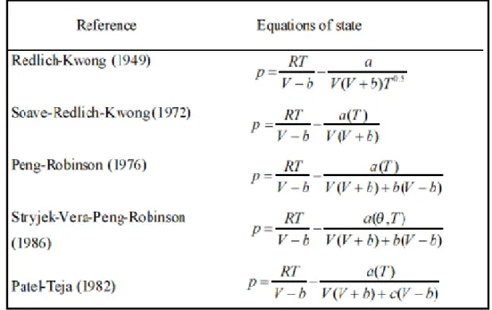
Realizing the limitations of the VDW, in 1994, Redlich and Kwong (RK) succeed in formulated two parameter cubic equation of state that improving hard sphere term and attractive term equation by proposing temperature dependence for the attractive term (Ashour et al., 2011). Hence, many investigators got interest in the EOS limitations by improving and modify VDW equations and improving RK equations, for example Soave in late 1972 and Peng-Robinson in 1976 proposed additional modifications for the RK equation to make the phase equilibria predictions are more accurate in order to predict vapour pressure, liquid density, and K-values or known as equilibrium ratios (Velderama, 2003). Since then, many works and experimental values had been done and more additional theory to prove the existence theorem of hydrogen bonding have been developed, for example thermodynamic perturbation theory (TPT) that was proposed by Wertheim in late 1987 (Velderama, 2003).
In 1980, Van Konyenburg and Scott successfully demonstrated the most critical equilibria exhibited by binary mixtures that could be qualitatively predicted by the VDW EOS that is fully limited and rarely accurate for describing critical properties and phase equilibria calculations as explained by Velderama (Velderama, 2003).
Five examples of cubic equations of state on the VDW equations are listed in Figure 2.1.
10
Figure 2. 1: Five Examples of Improved Cubic EOS from the VDW EOS (Velderama, 2003)
From figure 2.1, RK EOS equation is quite similar to the SRK, except that Soave introduced new constant for replacing the term a/T0.5 with a general temperature dependent term a(T) as in the SRK equations above and he also introduces an accentric factor. The validity of the SRK fitted well with the experimental that had been done by him and several researches like Zheng and Daubert in predicting phase behaviour of mixtures in the critical region using mixtures of hydrocarbons in estimating their critical properties (Velderama, 2003). From here, it is clear that RK- EOS cannot predict the critical properties of the phase equilibria mixtures and only suitable for moderate temperatures and pressures. Yet the fundamentals introduction of the accentric terms gives an improvement in fluid equilibria predictions in hydrocarbon mixtures.
For the PR EOS, in late 1976, they slightly improve the predictions of fluid volumes and critical compressibility factor and Ashour reported that PR-EOS functions is excellent in characterizing non hydrocarbon components like hydrogen and nitrogen containing mixtures (Ashour et al., 2011). Ashour in his paper explains that PR-EOS gives good result in obtaining a relatively accurate, non-iterative and computationally efficient correlation of high pressure mixtures used in gas turbines and rocket engines. Ashour also states in his paper that SRK EOS fails to predict liquid compressibility accurately and comparisons of vapour pressure calculation
11
that had been done shows small error in both equations when comparing with the experimental results He added that PR-EOS enjoys more simplicity and reliability than other EOS functions but both PR and SRK break down at C10 to C11 and heavier compounds (Ashour et al., 2011). However, the successes of both EOS are restricted to the estimation of phase equilibria pressure as depicted in figure 2.2.
Figure 2.2 describes that, for the mixture’s property calculation, none single EOS are capable in the prediction and calculation mixture’s property where the calculated saturated liquid volumes are not been improvised and tend to be higher than the experimental data.
As years by years, there are many complex and accurate EOS have been introduced and published for better understanding in PVT properties and VLE. Velderama outlined in his article that summarized some basic rules that should be observed for developing molecular based EOS as in Figures 2.2 and 2.3 below. It can be concluded from here that the mixtures polarity by means of non hydrocarbon and hydrocarbon mixtures and equilibrium condition give a very significant impact on the calculation of the VLE and mixtures phase equilibria. Not all EOS functions can be applied. From Figure 2.3, most of the recommendations lead to SRK, PR, and PTV as the best EOS functions in describing the fluid behaviour. Thus, this is one of the reasons on why this study trying to use SRK and PR for describing phase envelope with varies natural gas mixtures with different non-hydrocarbon compositions.
12
Figure 2. 2: Recommendations on Suitability of Modelling Mixtures by EOS (Velderama, 2003)
Figure 2.3:Recommendation on General EOS and Mixing Rule for Different Types of Liquid-Vapor Mixtures (Velderama, 2003)
13
Figure 2.4: Selected Mixing Rule and Combining Rules Used In Two-Constant Cubic EOS (Velderama, 2003)
It is said by Ashour that the most applicable EOS functions in fluid characterization in terms of phase equilibria is RK-EOS, SRK-EOS and PR-EOS because both SRK and PR introduced accentric factor as the third parameter to obtain parameter a in their equations (Ashour et al., 2011).
The list of different mixing rules that can be used in EOS functions are presented in Figure 2.4. The recommendations presented in figure 2.3 above is an indication that for the fluid mixtures used in this study, most hydrocarbon phase equilibria calculations will be predicted accurately by using SRK, PRSV, PR and by using VDW mixing rule of one parameter or two parameter binary interactions as shown in Figure 2.4. As can be seen from Tables 4.1 to 4.2, the compositions used in this study ranging from a mixtures of a polar and non polar components which depicted that another possible mixing rule to be used as indicated in Figure 2.3 and 2.4 which is WS mixing rule that is recommended to be applicable at low pressure of less than 10 atm. The risk is worth taking on trying to use WS mixing rules by using the cubic EOS functions in getting an understanding of the outcomes result.
14
With regards to the natural gas mixtures discussed earlier in this studies, Hartono describes that for modelling systems with non-polar and slightly polar compounds, a new concept has evolved in recent years with the introduction of EOS abbreviated CPA (Cubic Plus Association) presented by Kontogeorgis in 1996 that used for modelling VLE for alcohol-hydrocarbon system in correlating LLE for this mixtures.
CPA models are actually combining the physical effects from the classical models and a chemical contribution (Hartono et al., 2004).
Kontogeorgis describes that CPA is the combination of the physical term and the association term. The physical terms characterized as repulsive forces and attractive forces and can be calculated by using simple EOS models like SRK and PR. The association term accounts for the hydrogen bonding and calculated from the Weirtheim perturbation theory (Kontogeorgis et al., 1996). He added that perturbation theory are complex and endless that depending on the nature of the system. That is why the needs of reference state, approximations and simple methods are needed in account for the perturbation theory (Kontogeorgis et al., 2010).
Kontogeorgis and his friends added the term “pseudo-association” which refered as previously mention reference system for accounting the limitations of the perturbation theory. They pointed that for strongly dipolar molecules like acetone or a quadrupolar like carbon dioxide, these molecules are treated using the concept of pseudo-association that actually being able to act as associating compounds (Kontogeorgis et al., 1996, 2010). This approach renders CPA to be reliable to such compounds without the need of extra terms to account for polar or quadropolar interactions. And for the needs of understanding, it is worth evaluating phase behaviour of natural gas by using CPA EOS models.
The use of non quadratic mixing rules for the prediction of VLE in polar organic binary solutions, which had been discussed in details by Vahid. His research used the combination of cubic EOS and excess free Gibbs energy mixing rules in representing the behaviour of highly polar solutions. Vahid states that the combined EOS and free Gibbs energy models need to reproduce the excess Gibbs free energy models as closely as possible in order to represent low pressure VLE of polar mixtures accurately and to make vapor liquid predictions at higher temperatures and pressures accurate using only low pressure information. In his work, the introduction of two
15
models Gibbs free energy is used which were UNIQUAC and NRTL models and both models are in good association only with WS mixing rules where NRTL model has weak predictive capabilities due to the limitation in temperature-dependent variables and UNIQUAC has better approximations for prediction of polar organic mixtures (Vahid, 2004).
Velderama in his papers describes that quadratic mixing rules are usually sufficient for the correlation of phase equilibrium in simple systems. Velderama describes that, to treat more complex systems, there is a modifications by previous researcher that introduced a second interaction parameter by making the binary interaction parameter concentration dependent, thus transforming mixing rule in a non-quadratic form (Velderama, 2003)
He also added that EOS + Gibbs Free energy seems to be the most appropriate for modelling mixtures with highly asymmetric components which had been applied in Huron and Vidal that modelling the combination of EOS and Gibbs free energy to modelling a mixtures of low and high pressure vapor liquid mixtures, to liquid-liquid equilibrium, and gas solid equilibria, with the important contribution of mixing rules such as WS. Velderama shared an important predictions of the WS mixing rule, where this mixing rule has been the focus of several studies, and among all the mixing rule that had been tested by several authors that combining NRTL and UNIQUAC models for the excess Gibbs free energy and the study shows that for strongly polar-non-polar mixtures, the combination of WS + NRTL gives the best results and the combination of WS + UNIQUAC models give best results in strongly polar + strongly polar mixtures. This gives an early estimation that EOS +Gibbs Energy+ mixing rule are not capable in predictions of any hydrocarbon mixtures (Velderama, 2003).
In relevance of the introduction of CPA-EOS-NRTL-mixing rule into this studies by combining equation of state of PR and RK families is that the capabilities of the equation in modelling mixtures of varies pressure range and also a temperature dependence and expected that some equations introduced in this study that use CPA+EOS+mixing rule and EOS+ Gibbs free energy mixing rule like CPA-PR- VDW, CPA-SRK-VDW, PR-UNIQUAC-WS and PR-NRTL-WS will gives an
16
interesting results in modelling natural gas mixtures phase behaviours. Some general formulations on each EOS models described are presented in Table 2.1.
17
Table 2. 1: Summaries of the General Formalism of Eight EOS Models Abbreviation
[a,b,c,]
General Formalism[a,b,c,]
a[a,b,c,] b
[a,b,c,]
a(T)[a,b,c,] Mixing Rule[a,b,c,]
PR-VDW P =RT/(V–b)
+acα(Tr)/(V(V+b))
0.45724(R2(Tc)2) /Pc
0.077 80RT c/Pc
[1 + (0.37464 + 1.5 4226ω – 0.26992ω2)(1–
(Tr)1/2)]2
a = ∑∑xixjaij ; aij = √((aiaj)(1-kij)) b = ∑∑xixjbij ; bij = ½(bi + bj)(1-βij)
PR-WS P =RT/(V–b)
+acα(Tr)/(V(V+b))
0.45724(R2(Tc)2) /Pc
0.077 80RT c/Pc
[1 + (0.37464 + 1.5 4226ω – 0.26992ω2)(1–
(Tr)1/2)]2
a = b[∑xiai/bi- A∞E(x)/ Ω] b = ∑∑xixj(b - a/RT)ij/[1 -∑ xiai/biRT -
A∞E(x)/ΩRT]
SRK-VDW P =RT/(V–b)
+acα(Tr)/(V(V+b))
0.42748(R2(Tc)2) /Pc
0.086 64RT c/Pc
[1 + (0.480 + 1.574ω – 0.176ω2)(1–
(Tr)1/2)]2
a = ∑∑xixjaij ; aij = √((aiaj)(1-kij)) b = ∑∑xixjbij ; bij = ½(bi + bj)(1-βij)
SRK-EXT-
VDW P =RT/(V–b)
+acα(Tr)/(V(V+b))
0.42748(R2(Tc)2) /Pc
0.086 64RT c/Pc
[1 + (0.48508 + 1.55171ω – 0.15613ω2)(1–
(Tr)1/2)]2
a = ∑∑xixjaij ; aij = √((aiaj)(1-kij)) b = ∑∑xixjbij ; bij = ½(bi + bj)(1-βij)
CPA-PR- VDW
P=RT/(V-b) - (a/(V(V+b)) + (RT/V)
ƿ∑[1/XA – 0.5][∂XA/∂ƿ]
0.45724(R2(Tc)2) /Pc
0.077 80RT c/Pc
[1 + (0.37464 + 1.5 4226ω – 0.26992ω2)(1–
(Tr)1/2)]2
a = ∑∑xixjaij ; aij = √((aiaj)(1-kij)) b = ∑∑xixjbij ; bij = ½(bi + bj)(1-βij)
CPA-SRK-
VDW P=RT/(V-b) -
(a/(V(V+b)) + (RT/V) ƿ∑[1/XA – 0.5][∂XA/∂ƿ]
0.42748(R2(Tc)2) /Pc
0.086 64RT c/Pc
[1 + (0.480 + 1.574ω – 0.176ω2)(1–
(Tr)1/2)]2
a = ∑∑xixjaij ; aij = √((aiaj)(1-kij)) b = ∑∑xixjbij ; bij = ½(bi + bj)(1-βij)
18 PR-NRTL-
WS
P =RT/(V–b) +acα(Tr)/(V(V+b))
a=b[g E0 /A1 +∑x1(ai/bi)+RT/
Ai∑xiln(b/bi)]
b=∑
bi xi [1 + (0.37464 + 1.5 4226ω – 0.26992ω2)(1–
(Tr)1/2)]2
a = b[∑xiai/bi- A∞E(x)/ Ω]
b = ∑∑xixj(b - a/RT)ij/[1 -∑ xiai/biRT -
A∞E(x)/ΩRT]
0.45724(R2(Tc)2) /Pc
0.077 80RT c/Pc
(b - a/RT)ij = 0.5[bi(1 - li) + bj] - (aiaj)0.5(1 - kij)/RT ; li ≠0 for all solutes and lj=0 for all solvents
PR- UNIQUAC-
WS
P =RT/(V–b) +acα(Tr)/(V(V+b))
a=b[g E0 /A1 +∑x1(ai/bi)+RT/
Ai∑xiln(b/bi)]
b=∑
bi xi [1 + (0.37464 + 1.5 4226ω – 0.26992ω2)(1–
(Tr)1/2)]2
a = b[∑xiai/bi- A∞E(x)/ Ω] b = ∑∑xixj(b - a/RT)ij/[1 -∑ xiai/biRT -
A∞E(x)/ΩRT]
0.45724(R2(Tc)2) /Pc
0.077 80RT c/Pc
(b - a/RT)ij = 0.5[bi(1 - li) + bj] - (aiaj)0.5(1 - kij)/RT ; li ≠0 for all solutes and lj=0 for all solvents [a] Kontogeorgis et al., 1996
[b] Velderama, 2003 [c] Velderama et al., 2003 [d] Diamantonis et al., 2013
19
2.4: About PRODE software in Microsoft Excel Simulation
The attention for using simulator is an added advantage in testing different sets of natural gas mixtures phase envelope by using EOS models. The idea is that, engineers should be able to choose which equation is right for modelling thermodynamic properties and phase envelope of the mixtures, and by using simulator like Prode properties is another way of conducting, validating and testing each EOS models for different sets of mixture. Another reasons on why testing EOS models by using Prode is that most of the engineers and students should use the equations for application of the industrial usage that was developed an invented by previous scientist and mathematician. It was many EOS models that were developed these days and very few of the usage limitation of each equation are reported and their applicability and efficiency for certain mixtures is still questionable.
Prode properties includes a comprehensive collection of procedures that used to solve problems related to physical properties data, heat and material balance, process simulation, process control, equipment design, phase envelope calculations, flash calculation, separations, instrument design and more.
The technical features overview of the Prode Properties includes direct access from Windows applications that includes Microsoft Excel and Visual Studio applications that includes MATLAB, MathCad and more. The properties of this software support for up to 500 different streams up to 100 components per stream.
In relation to the thermodynamic properties calculation, a Prode property includes several compilations of chemical data and Binary Interaction Parameters (BIPs) are available. A comprehensive set of thermodynamic models likes Regular, Wilson, NRTL, UNIQUAC, UNIFAC, Soave-Redlich-Kwong, Peng-Robinson, BWRS, Steam Tables (IAPWS 1995), Lee Kesler Plocker , AGA (ISO 20765); GERG (ISO 18453); GERG (2008); Hydrates (VDW-Platteeuw), models which include association contribute CPA SRK, CPA PR, PC-SAFT, EOS models with different mixing rules like Van der Waals, Huron Vidal and Wong Sandler are also available for the ease of industrial applications.
The software also have a functions for thermodynamic calculation such as enthalpy and entropy and also coded built ins models for industrial applications in performing
20
a set of flash operations at isothermal, isobaric, isochoric and adiabatic. In relation to the modeling mixtures of different compositions in performing phase envelope calculations, Prode properties include functions for calculating specific properties of mixtures that includes critical point, cricodentherm, cricondenbar, and cloud point.
Here after, the limitation of this software is that the developer doesn’t share on details about the coding built in for generation of the calculation that similarly observed as others commercial software such as PVTi, VLE flash and HYSYS.
21
CHAPTER 3
METHODOLOGY
3. 1: Introduction
Procedure identification of this studies are modelling phase envelopes of various sets of data that comprise of twenty four contextual mixtures by using excel simulator Prode add in. The procedure in this modelling is simple and tested 200 equations of state is not a problem, but the idea is that which existing equations of state are capable of characterizing natural gas mixtures with and without non-hydrocarbon components with a minimum percentage AAD.
3. 2: Procedure
The steps involve in this modelling is the same as we do modelling in every other software like PVTi, VLE and HYSYS. As described in chapter two, twenty four mixtures of natural gases will be modelled by using this simulator and the resulted temperature and pressure of the modelled phase envelope are compared with the experimental pressure and temperature obtain from the literature. Then, all sets of data in terms of deviation pressure calculated and temperature calculated to the experimental values are calculated and presented in terms of the average arithmetic deviation or AAD. In this case, two types of percentage AAD will be presented which is percentage AAD due to temperature and pressure. The significance of calculating both percentages AAD is that, most of the EOSs are good at predicting and modelling phase envelope with respect to temperature deviation, but for pressure deviation, it entirely varies.
Due to lots of data calculated for temperature and pressure and for matching between calculated values to the experimental values, the easiest way is to use excel formulae as equation 3.5 and the matching values were used to calculate percentage deviation.
The calculated percentage deviation formulae used for temperature and pressure deviation are as equation 3.1, 3.2 and for percentage AAD by using equation 3.3 and 3.4.
22
% 𝑫𝒆𝒗 = 𝟏𝟎𝟎 𝒂𝒃𝒔 𝒄𝒂𝒍𝒄𝒖𝒍𝒂𝒕𝒆𝒅 𝑷−𝒆𝒙𝒑𝒆𝒓𝒊𝒎𝒆𝒏𝒕𝒂𝒍 𝑷
𝒆𝒙𝒑𝒆𝒓𝒊𝒎𝒆𝒏𝒕𝒂𝒍 𝑷 (3. 1)
% 𝑫𝒆𝒗 = 𝟏𝟎𝟎 𝒂𝒃𝒔 𝒄𝒂𝒍𝒄𝒖𝒍𝒂𝒕𝒆𝒅 𝑻−𝒆𝒙𝒑𝒆𝒓𝒊𝒎𝒆𝒏𝒕𝒂𝒍 𝑻
𝒆𝒙𝒑𝒆𝒓𝒊𝒎𝒆𝒏𝒕𝒂𝒍 𝑻 (3. 2)
%𝑨𝑨𝑫 𝑻 = 𝟏𝟎𝟎𝒏 𝒂𝒃𝒔 𝒄𝒂𝒍𝒄𝒖𝒍𝒂𝒕𝒆𝒅 𝑻−𝒆𝒙𝒑𝒆𝒓𝒊𝒎𝒆𝒏𝒕𝒂𝒍 𝑻 𝒆𝒙𝒑𝒆𝒓𝒊𝒎𝒆𝒏𝒕𝒂𝒍 𝑻
𝒏𝒊=𝟏 (3. 3)
%𝑨𝑨𝑫 𝑷 = 𝟏𝟎𝟎𝒏 𝒂𝒃𝒔 𝒄𝒂𝒍𝒄𝒖𝒍𝒂𝒕𝒆𝒅 𝑷−𝒆𝒙𝒑𝒆𝒓𝒊𝒎𝒆𝒏𝒕𝒂𝒍 𝑷 𝒆𝒙𝒑𝒆𝒓𝒊𝒎𝒆𝒏𝒕𝒂𝒍 𝑷
𝒏𝒊=𝟏 (3. 4)
INDEX(E:E,MATCH(MIN(ABS(E:E-C3)),ABS(E:E-C3),0)) (3. 5) Where;
E and C = Excel Column ABS =Absolute
MIN =Minimum
23 3.3: Procedure Summary
Summaries of the steps involve for calculation of the phase behaviours for 24 natural gas mixtures as in Table 4.1 and 4.2 by using eight EOSs models are listed below:
1. One EOS model and natural gas mixture had defined in the Prode add in simulator; note that only a mixture and one EOS models could be tested at the same time.
2. Particular isothermal conditions for simulation were defined where in this case at STP.
3. The simulation should be running after all the parameters and natural gas composition had defined and resulted graph of phase envelope with its calculated values of temperature and pressure are analysed.
4. Then, the resulted temperature and pressure values together with the experimental values will be match in the excel file by using equation 3.5.
5. The values match for temperature and pressure are used to calculate percentage deviation by using equation 3.1 and 3.2.
6. Percentage AAD of T and P from the step 5 were calculated by using equation 3.3 and 3.4 for that particular mixture.
7. The calculated values of T and P from step 3 together with experimental values were plotted on the same graphs.
8. Step 1 to step 6 were repeated for another 7 EOS models for same mixtures in this study.
9. Steps 1 to 7 were repeated for another 23 natural gas mixtures.
10. The resulted percentage AAD of T and P calculated were compared and analysed in choosing the most applicable EOS models for modelling that particular natural gas mixture.
11. Resulted graph generated will be 192 graphs as shown in the appendices.
24
CHAPTER 4
RESULTS AND DISCUSSIONS
4.1: Introduction
There are twenty four types of natural gas mixtures used in this, study with different component compositions. These can be divided into different sets of analysis which is set 6, set 9, set 15, set 18, set 19 and set 20. The different sets of the mixtures composition were obtain from the literature studies conducted previously by different authors that modelling and investigating various thermodynamics calculation theories for different types of equations of state. The summaries of different sets of data are presented as in Tables 4.1 and 4.2.
There are 192 graphs of natural gas mixture’s phase envelope generated for different equation of states and presented in the appendix. But for the ease of presentation and comparing, the graphs is combine and yielded 24 phase envelope graphs as shown below and table summarizes of the experimental values, calculated values and the percentage AAD for temperature and pressure presented in Tables 4.3 to 4.8. The resulted graph presented in this chapter will be briefly discussed.
25
Table 4. 1: Summaries of Composition of Natural Gas Mixtures Used In This Study component
mixture
SET 6 [a] SET 9[b] SET 15[c]
SNG 2 SNG 3 SNG 4 GAS 1 GAS 1 GAS 2 GAS 3 SNG 1 SNG 2 SNG 3 SNG 4 SNG 5
nitrogen 1.70% 1.71% - 1.70% - 6.90% 0.75% - - - - -
carbon dioxide 1.71% 1.70% - 1.70% - 0.51% 3.91% - - - - -
methane 89.99% 89.98% 90.00% 89.98% 89.00% 88.19% 70.20% 93.51% 84.28% 96.61% 94.09% 93.60%
ethane 3.15% 2.86% 4.57% 3.01% 7.00% 2.72% 9.22% 2.97% 10.07% - 4.47% 2.63%
propane 1.58% 1.43% 2.24% 1.51% - 0.85% 2.76% 1.01% 4.03% - - -
iso-butane 0.78% 0.71% 1.14% 0.75% - 0.17% 0.66% 1.05% 0.60% 1.53% - 1.49%
n-butane 0.79% 0.72% 1.15% 0.75% 4.00% 0.32% 0.98% 1.47% 1.03% 1.48% - 1.49%
iso-pentane 0.15% 0.45% 0.45% 0.30% - 0.09% 0.40% - - 0.39% 1.45% 0.80%
n-pentane 0.15% 0.45% 0.45% 0.30% - 0.09% 0.42% - - - - -
n-hexane - - - 0.12% 0.82% - - - - -
n-heptane - - - 0.03% 9.87% - - - - -
n-octane - - - 0.02% - - - -
SUM/ % Mol 100% 100% 100% 100% 100% 100% 100% 100% 100% 100% 100% 100%
[a] Atilhan et al., 2011 [b] Atilhan et al., 2011 [c] Nasrifar et al., 2006
26
Table 4. 2: Summaries of Composition Natural Gas Mixtures Used In This Study component
mixture
SET 18[d] SET 19[e] SET 20[f]
SNG 1
SNG 2
SNG 3
SNG 4
SNG 5
GAS 1
GAS 2
MIXTURE A
MIXTURE B
MIXTURE C
MIXTURE D
MIXTURE E
nitrogen 1.56% 0.31% 0.77% 6.90% 5.65% - - - - 0.86% 0.80% 0.60%
carbon dioxide
25.91
% 0.20% 1.70% 0.51% 0.28% 95% 99% - - - - -
methane 69.11
%
90.48
%
84.45
%
88.19
%
83.35
% - - 85.34% 75.44% 75.70% 74.27% 90.07%
ethane 2.62% 8.04% 8.68% 2.72% 7.53% - - 7.90% 15.40% 13.59% 16.51% 6.54%
propane 0.42% 0.80% 3.30% 0.85% 2.01% 5% - 4.73% 6.95% 6.74% 6.55% 2.20%
iso-butane 0.11% 0.08% 0.29% 0.17% 0.31% - - 0.85% 0.98% 1.34% 0.84% 0.29%
n-butane 0.10% 0.12% 0.59% 0.32% 0.52% - 1% 0.99% 1.06% 1.33% 0.89% 0.28%
iso-pentane 0.03% 0.01% 0.08% 0.09% 0.12% - - 0.10% 0.09% 0.22% 0.07% 0.01%
n-pentane 0.02% 0.01% 0.09% 0.09% 0.14% - - 0.09% 0.08% 0.22% 0.07% 0.01%
n-hexane 0.11% 0.00% 0.05% 0.12% 0.07% - - - -
n-heptane - 0.00% - 0.03% 0.01% - - - -
n-octane - - - 0.02% 0.01% - - - -
SUM/ %
Mol 100% 100% 100% 100% 100% 100% 100% 100% 100% 100% 100% 100%
[d] Nasrifar, et al.; 2005 [e] Gil, et al.; 2006 [f] Nasrifar, et al.; 2002
27
Table 4. 3: Comparison Table of Different EOS and Their Percentage AAD to the Experimental Values for Set 6 Type of EOS MIXTURE Experimental T
Range (K)
Experimental P Range (MPa)
Calculated T Range (K)
Calculated P Range
(MPa) %AAD/P %AAD/T
CPA-PR- VDW
SNG2 224.81 to 245.28 7.51179 to 1.57178 205.069 to 211.32 0.1013 to 6.4087 2.84% 0.13%
SNG3 239.31 to 270.6 9.68088 to 3.3032 214.202 to 211.236 0.1013 to 6.5889 5.40% 0.91%
SNG4 265.6 to 274.23 11.76229 to 1.59253 241.89 to 245.64 0.101327 to 0.532805 89.12% 12.84%
CPA-SRK- VDW
SNG2 224.81 to 245.28 7.51179 to 1.57178 207.319 to 217.883 0.10132 to 7.194 2.37% 0.33%
SNG3 239.31 to 270.6 9.68088 to 3.3032 217.36 to 218.06 0.101327 to 7.423 1.78% 0.18%
SNG4 265.6 to 274.23 11.76229 to 1.59253 218.81 to 226.13 0.101327 to 8.02 6.15% 0.68%
PR-VDW
SNG2 224.81 to 245.28 7.51179 to 1.57178 204.718 to 211.651 0.10132 to 6.711 2.94% 0.19%
SNG3 239.31 to 270.6 9.68088 to 3.3032 213.82 to 211.73 0.101327 to 6.92 3.47% 0.70%
SNG4 265.6 to 274.23 11.76229 to 1.59253 215.66 to 219.36 0.101327 to 7.52 7.41% 1.63%
SRK-VDW
SNG2 224.81 to 245.28 7.51179 to 1.57178 207.0907 to 212.077 0.10132 to 6.8308 3.04% 0.27%
SNG3 239.31 to 270.6 9.68088 to 3.3032 217.48 to 211.74 0.101327 to 7.00 2.29% 0.32%
SNG4 265.6 to 274.23 11.76229 to 1.59253 218.74 to 252.59 0.101327 to 9.80 6.74% 0.98%
PR- UNIQUAC-
WS
SNG2 224.81 to 245.28 7.51179 to 1.57178 209.449 to 205.79 0.10132 to 4.093 8.28% 0.64%
SNG3 239.31 to 270.6 9.68088 to 3.3032 217.67 to 207.59 0.101327 to 4.01 19.66% 2.53%
SNG4 265.6 to 274.23 11.76229 to 1.59253 219.75 to 213.14 0.101327 to 3.90 21.47% 4.41%
PR-NRTL-WS
SNG2 224.81 to 245.28 7.51179 to 1.57178 204.698 to 231.4953 0.10132 to 6.5224 7.44% 1.49%
SNG3 239.31 to 270.6 9.68088 to 3.3032 215.36 to 226.82 0.101327 to 6.76 17.28% 3.62%
SNG4 265.6 to 274.23 11.76229 to 1.59253 216.48 to 243.62 0.101327 to 6.56 21.05% 6.19%
SRK-EXT- VDW
SNG2 224.81 to 245.28 7.51179 to 1.57178 206.256 to 217.049 0.10132 to 7.149 2.33% 0.17%
SNG3 239.31 to 270.6 9.68088 to 3.3032 216.74 to 217.37 0.101327 to 7.39 2.03% 0.19%
SNG4 265.6 to 274.23 11.76229 to 1.59253 217.99 to 226.28 0.101327 to 8.03 6.40% 0.80%
PR-WS SNG2 224.81 to 245.28 7.51179 to 1.57178 209.460 to 226.8026 0.10132 to 6.555 6.90% 1.08%