Thus, many researchers have resorted to using machine learning models to overcome this pitfall of the PM model. The results showed that the ensemble based on WOA-ELM (WOA-ELM-E) improved the performance of the baseline models in general. WOA-ELM-E was the best model at most meteorological stations.
General Introduction
Recent developments in computing technologies allow the application of machine learning to estimate ET. The machine learning models have consistently shown promising performance in estimating ET0, not to mention that many of the empirical models or equations outperformed them. Nevertheless, the locality characteristic still exists in most of the developed machine learning models reported in the literature.
Problem Statement
In addition, qualitative hunger can also be reflected from the locality characteristics of the machine learning models. Many machine learning models can only be trained and tested in situ, which means that the spatial robustness of the models is quite poor. In other words, the prerequisite for a workable machine learning model is the existence of different features in the input.
Aim and Objectives
To minimize computational costs, data fusion techniques were integrated with the three selected basic improvisation basic models. The three elementary basic models selected are the MLP, SVM and ANFIS for their suitability in regression analysis. The bootstrap aggregation (data-centric), Bayesian modeling approach (model-centric), and NNE approaches were chosen as the data fusion techniques to be integrated into the base models.
Contribution of the Study
Proper implementation of these plans can help catalyze the growth of the agricultural sector. This can stimulate both the recovery and the resilience of the national economy, which has unfortunately been dwindling in recent years. The well-being of the society can be further improved to spur Malaysia to become a high-income country in the near future.
Thesis Structure
Evapotranspiration
Non-weighable lysimeters are usually used for long-term monitoring, while the weighable lysimeters give measurements with finer temporal resolution (Wang and Dickinson, 2012). In fact, studies related to the ET estimation often used the measurements of lysimeters as the calibration standard (Anapalli, et al., 2016; Liu, et al., 2017). The scarcity and availability of lysimeters also limits their coverage and hinders the easy measurement of ET in different locations (Stanhill, 2005).
Temperature-Based Models
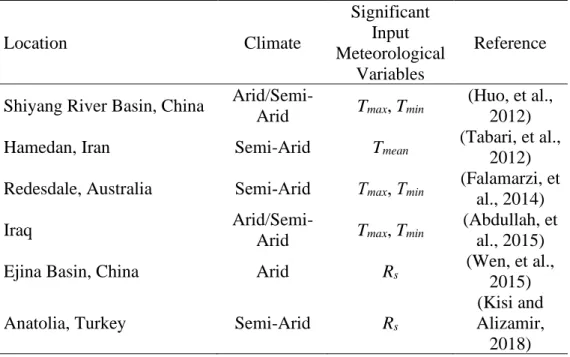
Temperature-based models used to calculate ET0 are generally modified or derived from the temperature-based model for potential evapotranspiration (PET). Essentially, temperature-based models measure atmospheric evaporative demand based on temperature data taken over a specific time scale. Among the temperature-based models, the Hargreaves-Samani (HS) model was developed and improvised in the 1980s (Hargreaves and Samani, 1985).
Radiation-Based Models
The first radiation-based model can be traced back to the Ritchie model developed in the 1970s (Ritchie, 1972). However, the performance of the Ritchie model still lags far behind modern techniques such as the ANFIS (Gonzalez del Cerro, et al., 2021). This indicated that the Ritchie model, besides being a convenient alternative, cannot be considered the first choice solution for ET0 estimation.
Combinatory Models
The PM model is considered one of the most popular models in ET0 estimation. The PM model includes most of the input meteorological variables believed to explain ET0 well. Therefore, a list of supporting equations and assumptions is needed to complement the PM model (Valiantzas, 2013).
Machine Learning for Evapotranspiration
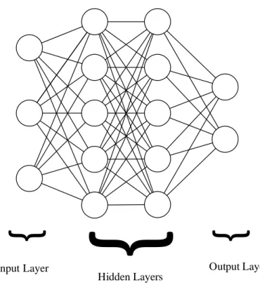
- Artificial Neural Network
- Support Vector Machine
- Fuzzy Logic
- Other Models
The application of ANN is a simulation of biological neurons in the nervous system, where neurons are connected via synapses. The purpose of the study was to obtain information on evapotranspiration in the future generation. The most pronounced characteristic of the current research culture is the use of hybrid machine learning models.
ANFIS
ANFIS S-ANFIS
- Data Fusion
- Bayesian Modelling Approaches
- Ensemble Model for Evapotranspiration
- Metaheuristic Approach
- Research Flow Chart
- Data Acquisition
- Normalisation of Data
- K-Fold Cross-Validation
- Input Combinations
- Multilayer Perceptron
- Adaptive Neuro-Fuzzy Inference System
- Data Fusion
- Bootstrap Aggregating
- Bayesian Model Averaging
- Non-Linear Neural Ensemble
- Scenario 1: Training and Testing with Local Data
- Scenario 2: Estimation of ET 0 using Exogenous Models
- Scenario 3: Model with Pooled Global Data
- Performance Evaluation
- Mean Absolute Error
- Mean Absolute Percentage Error
- Coefficient of Determination
- Performance of Base Models at Different Stations
- Effect of Input Meteorological Variables
- Comparison of Base Models
- Data Fusion I: Bootstrap Aggregating
- Bootstrap Aggregating with SVM
- Bootstrap Aggregating with ANFIS
- Summary
- Data Fusion II: Bayesian Model Averaging
- Bayesian Weight
Similarly, bootstrap clustering has been used as a tool to improve the accuracy of ET0 estimation. Basically, iteration-based optimization works on improving the objective functions through a neighborhood search technique (Şen, Dönmez, & Yıldırım, 2020). Data fusion techniques were then used to improve the performance of the underlying machine learning models.
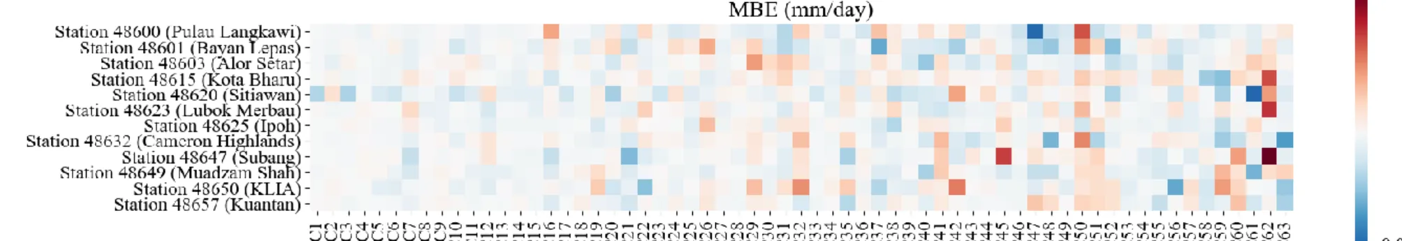
The chosen data fusion techniques targeted various possible pitfalls in the base models. The performance of SVM can be explained by examining the working mechanism of the model itself. Furthermore, the MBE of the ANFIS estimates appeared to be unaffected by the input combinations.
As can be seen in the figures, integrating the bootstrap aggregation to develop BSVM yielded daunting results. There was a clear pattern in the improvement (or degradation) of the BSVM's performance compared to the base SVM. This can be attributed to the overfitting of the BSVM when lesser meteorological variables were entered as inputs (C43, C44, C53 and C58), which was similar to the finding of other published work (Logue and Manandhar, 2018).
The increase in error statistics suggested that the accuracy of the BSVM was reduced. Nevertheless, these results showed that the bootstrap aggregating data fusion technique failed to improve the performance of the model. In fact, the cluster effect (as shown in input combination selection) was not evident in the case of the Bayesian weighting.
However, as the number of input meteorological variables decreased, the dominance of the MLP decreased accordingly. The Bayesian weight of ANFIS increased gradually as the number of input meteorological variables decreased.
Inter-Model Ensemble using BMA
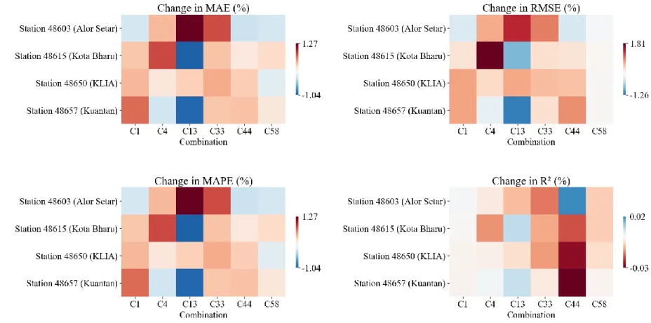
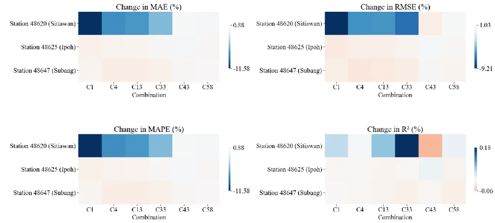
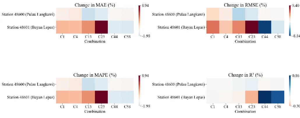
The performance of BMA-E in terms of MAE, RMSE, MAPE, R2 and MBE for stations in different groups is summarized in Figures 4.19 to 4.23. Compared with the baseline MLP, SVM, and ANFIS, BMA-E clearly improved ET0 estimation, as shown in Figures 4.19 to 4.23. There were several cases where the BMA algorithm was switched to BMS, as can be seen from the assignment of unit weights, the comparison of such BMA-E is less meaningful, since the resulting BMA-E only inherited the performance of the selected base models.
Attention will be given to the BMA-E where several base models were involved in the decision-making committee. For illustration purposes, the BMA-E was developed at Station 48603 (Alor Setar) using the C44 as the input combination selected for the detailed explanation. Although not remarkable, the BMA-E showed better performance compared to the base models in almost all aspects.
In addition, there were also some cases where only two of the base models were considered by the BMA algorithm. In this case, the BMA algorithm was 44.40% confident that the MLP was true, while the remaining 56.60% confidence was given to ANFIS (Bayesian weights can be referenced from Table 4.3). The BMA algorithm overruled the SVM in this case, possibly due to the extremely high MBE that may deteriorate the performance of BMA-E as a whole.
Therefore, just by comparing BMA-E with the basic MLP and ANFIS, the BMA data fusion technique has again proven its ability to improve ET0 performance based on the desired properties of the selected constituent base models.
Summary
This makes the resulting machine learning model (BMA-E) more explainable and can be studied with greater resolution by the scientific community. Nevertheless, the shortcomings of the BMA data fusion technique were also revealed through this research work. First, it is difficult for the BMA data fusion technique to include all the models as its constituents.
Consequently, some favorable properties of neglected or overlooked models are being sacrificed in the BMA-E development process. In most cases, this algorithm is reasonable to ensure optimal ensemble performance. However, this would also hinder the propagation of information extracted from the underlying models in the ensemble.
In other words, the rigid structure of the BMA data fusion technique lacks the flexibility to handle the noble characteristics of its possible constituent models. Second, the rigidity of the BMA data assimilation technique had resulted in many cases where the BMA-Es were not technically hybrid models or ensembles. This can be seen in many cases where a Bayesian weight of 1 is given to only one model (MLP in most cases).
Data Fusion III: Non-Linear Neural Ensemble
- WOA-ELM as Meta-Learner
- Inter-Model Ensemble using NNE
- Summary
- Performance of Exogenous Models (Scenario 2)
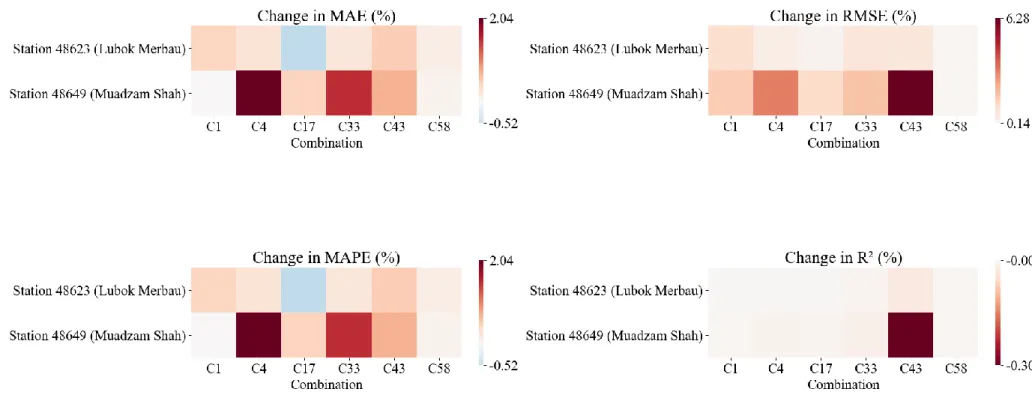
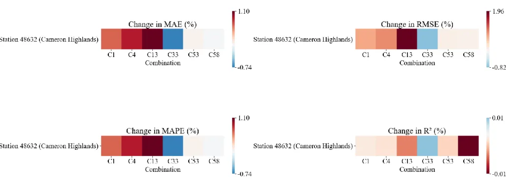
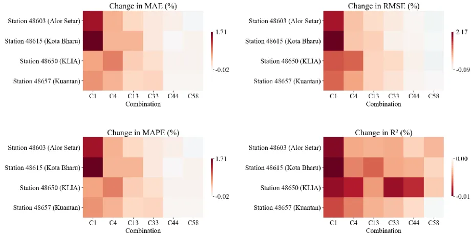
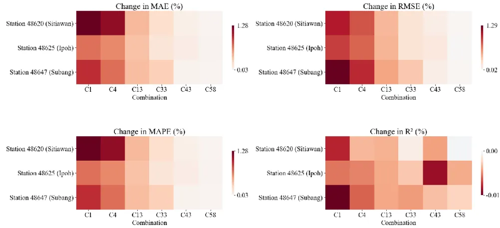
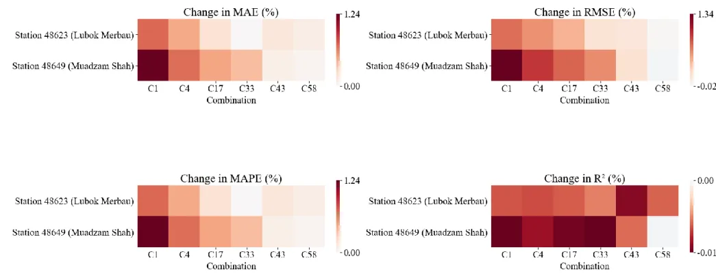
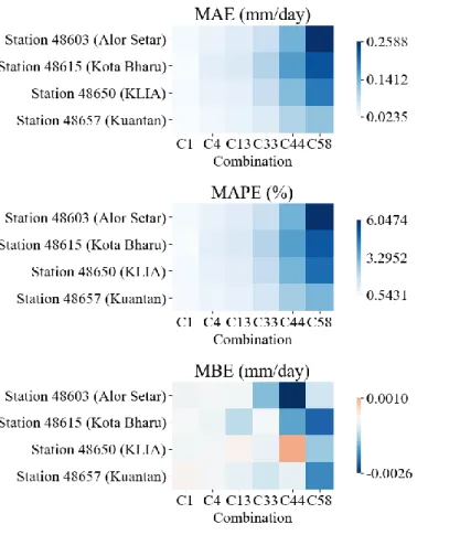
The performance of WOA-ELM-E, measured in terms of MAE, RMSE, MAPE, R2, and MBE, is presented as heat maps, as shown in Figures 4.24 to 4.28. Numerical values of the performance evaluation metrics are available in Appendix D (Table D1 - Table D5). Meanwhile, R2 of WOA-ELM-E was comparable to BMA-E, meaning that both ensembles match the data of each station well, considering different input combinations.
In this study, the GPI scores of the models were calculated based on the normalized values of the performance evaluation metrics against a different number of input meteorological variables. A comparison of the results of the GPI models developed in this research work (MLP, SVM, ANFIS, BMLP, BSVM, BANFIS, BMA-E and WOA-ELM-E) is shown in Figure 4.29 to Figure 4.33 (cluster 1 to cluster 5) . From Figures 4.29 to 4.33, WOA-ELM-E appears to be the most stable model, consistently maintaining in the upper class in terms of GPI values.
However, the performance of BMA-E was closely related to the performance of the baseline models, in which their poor performance would result in a poor BMA-E (Chen, et al., 2015). However, the performance of MLP and BMLP was not as stable as BMA-E or WOA-ELM-E. WOA-ELM-E was selected as the best ET0 estimation model at most stations, regardless of the number of input meteorological variables.
By reading horizontally, one can be informed about the performance of the best models trained at different stations as they were tested at other stations.