The undersigned confirm that they have read and nominate the Postgraduate Studies Program for acceptance of this thesis in order to fulfill the requirements for the degree indicated. Subsurface images of the area were then developed using the information from the seismic survey and borehole survey.
INTRODUCTION
- Introduction
- Study Area
- Geological Background
- Problem Statement
- Objectives
- Thesis Outline
The study area is surrounded by the robust buildings, industrial estate with offices and residential areas, which contributes to the noise pollution of the data. The same insight was applied to the standard penetration test (SPT), where the number of passes (N-value) of the test will increase with the hardness of the sample.
LITERATURE REVIEW
- Introduction
- Shallow Seismic Refraction
- The First Kick
- Interpretation Method
- Geophone Coupling Problem
- Noise Type
- Use of Seismic Refraction Survey
- Standard Penetration Test vs. Seismic Velocity
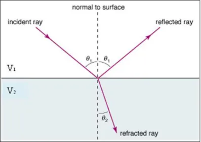
Both seismic waves return to the ground and the signal is received by the detector. The first arrival of the P waves indicates the travel time between the source and the detector.
METHODOLOGY
Introduction
Testing Acquisition Parameter
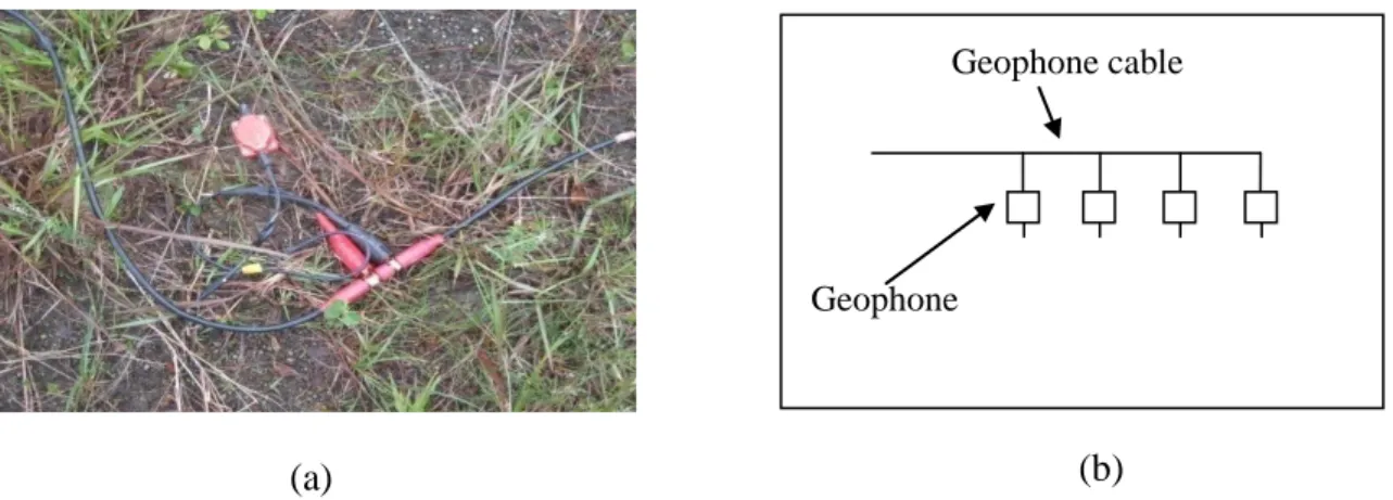
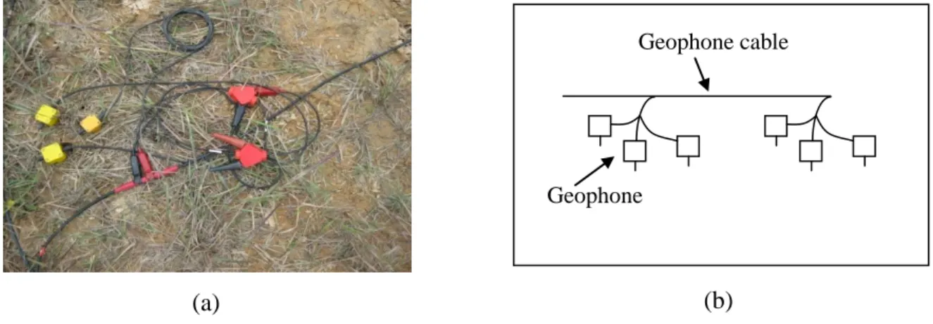
- Geophone Array Testing
- Source Testing
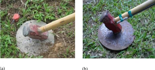
- Striker Plate
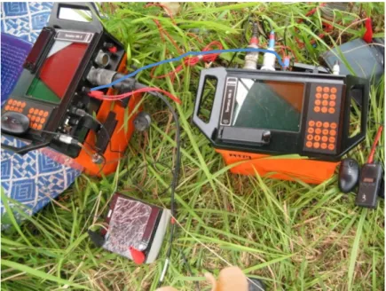
- Seismograph
- Trigger Type
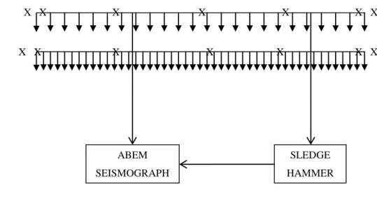
- Spread Layout and Shot Point Configuration System
But this source is very good and reliable for shallow acquisition, as it can summarize the ground movement and improve the waveforms of records after many shocks. The cost of the hammer is very cheap compared to other sources of induction power. Furthermore, the study area (urban area) precludes the use of dynamite or firecrackers.
These panels have been tested for their diameter, weight, thickness, durability against hammer blows, ability to give good signals and ductility of the material. The quality of the seismic signals is obtained by the impact energy of the impact hammer, the toughness of the impact plates against the impact of the impact hammer, and the mobility of the impact plate in the field. Two different seismographs are tested to determine the quality of the data provided by the equipment, the visibility of the first seismic signal, known as the first break, and the ability of the seismograph to accelerate the acquisition phase.
There are three parameters we look at the type of trigger during testing, there are 1) The sensitivity level of the trigger, 2) the time it takes to move the trigger from one point to another and 3) the time it takes to recover to the initial state. Since two different seismograph channels are used, two different alignment orientations are used. The firing point positions for the two seismographs are different since the geophonic space intervals are different.
Normal Processing Cycle
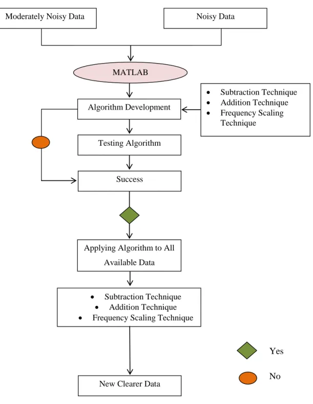
Advanced Data Improvement
- Subtraction and Addition Technique
- Frequency Scaling Technique
As a discriminative evidence of the noisy trace, the threshold value of this treatment is selected and fixed to 3. For any trace that has a threshold value greater than 3, the treatment will be applied to that trace. If the threshold value is less than 3, the trace will be preserved in its original state.
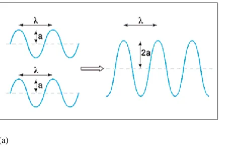
The new trace is the dot product of A(f) and each individual trace to be treated. To return the new traces to the frequency domain after treatment, inverse FFT is applied.
Correlation between Standard Penetration Tests (SPT) With Seismic
RESULTS AND DISCUSSIONS
Introduction
Acquisition Parameter Design for Noisy Area
- Geophone Array Testing
- Source Testing
- Striker Plate
- Trigger Type
- Equipment and Spread Layout
These arrays were tested to determine which array captured the most desired seismic signals. The important parameter of the impact plates in this study is the quality of the seismic signals obtained when the energy is transferred by the sledgehammer, the toughness of the impact plates compared to the impact of the sledgehammer and the mobility of the impact plates in the field . . The seismic signals from the entire strike plate are clear and the first fracture is visible.
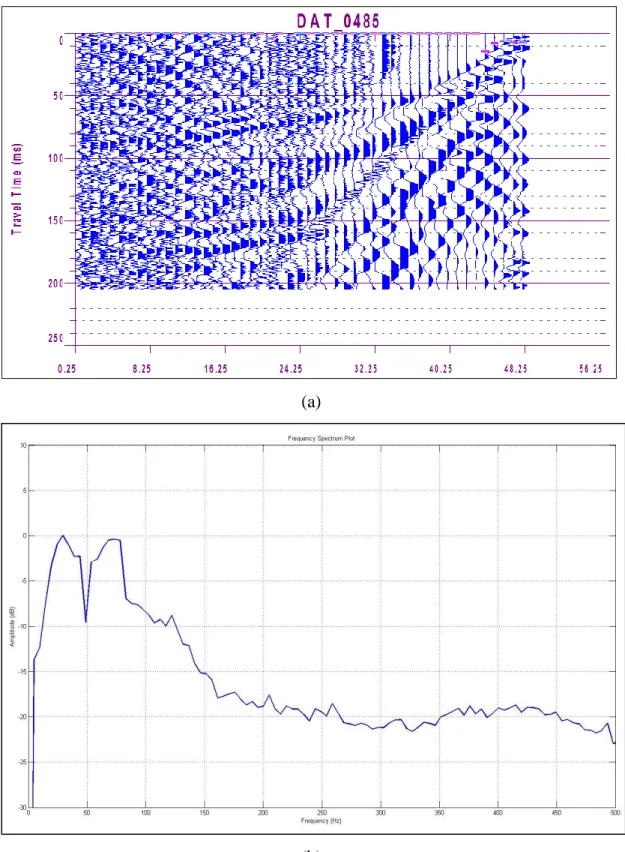
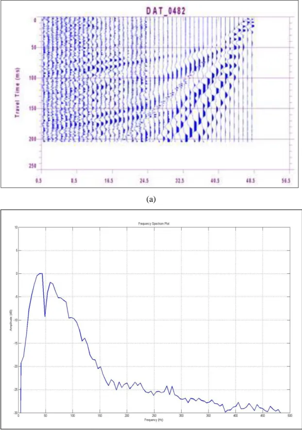
In order to compare the quality of the seismic signals obtained when the energy is transmitted by a jackhammer, we plotted the frequency spectrum for all the lightning strikes. The steel shock plate has a maximum amplitude of -32 dB at the low dominant frequency. The highest recorded amplitude of the high dominant frequency is at -1 dB for the wooden strike plate and -2.5 dB for the aluminum strike plate. Two different types of triggers were tested to determine the degree of sensitivity of the trigger, the time required to move the trigger from one point to another, and the time required to return to the initial position.
Although there is a difference in geophone spacing, both seismographs are still very useful in speeding up the recording process. Both seismograph systems were used in the recording phase as we have time constraints and must complete the work within the given time frame. From all the above tests, it is very important to design optimal parameters for seismic acquisition in urban areas.
Normal Processing Cycle
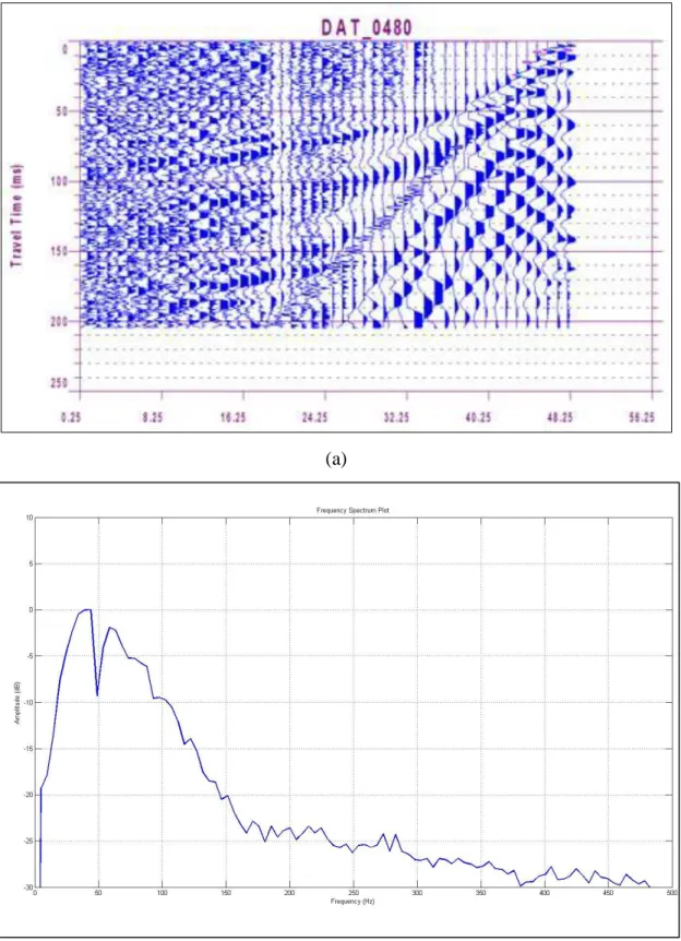
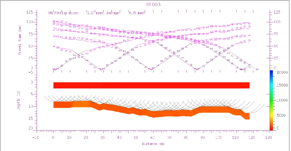
This seismic line has good seismic signal registration and the first break picking is easy as the first break is clearly visible on the recorded data. The depth to the refractor varies from 8.5 meters to 12.2 meters below ground with the time to the refractor in unit time varying from 15.4 milliseconds to 22.7 milliseconds. The assembly of first break picking for both models shows differences between manual picking and computerized picking.
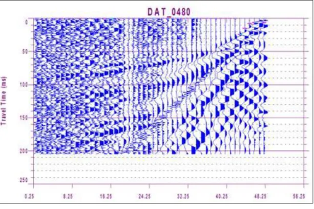
The records for each shot position of seismic line number 47 are shown in Figure 4.20 to Figure 4.25. From these figures, the noise contamination of these seismic lines is higher, thus making it difficult to choose the first break with confidence. A new proposed technique of noise reduction will be discussed in the next section to get better seismic signals focusing on the first break.
Good results were obtained with some data after undergoing the normal processing phase. Some data shows an error expected to arise from poor selection of the first fraction due to the bad trace being contaminated with noise. With this newly developed technique, it is hoped that the new result of the data will be better and there will be less noise contamination in the data.
Advanced Data Improvement
- Subtraction Technique and Addition Technique
- Frequency Scaling Technique
- Comparison between Subtraction and Addition Technique with
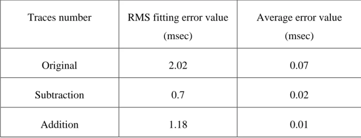
The lowest and highest difference is achieved by using track number 43 and track number 47 as the noisy track, respectively. Track numbers 42 and 45 give the same medium a different value when used as the noisy track. Then, the software processing is performed again using the seismic trace, after applying trace number 43 as the noisy trace.
From the 2D inverse model in Figure 4.37 and GRM interpreted depth model in Figure 4.38, the RMS fitting error value of the model is 1.40 and the average error value is 0.03. The noisy tracks, track number 40 to track number 48 are clearer as the noise on that track is greatly reduced and the first break signal is clearly seen. The 2D inverted model and GRM interpreted depth model after the software processing using the new seismic record with trace number 42 as the noisy trace are shown in Figure 4.40 and Figure 4.41 respectively.
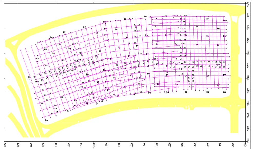
When seismic trace number 47 is used, the result of the 2D inverted model and the interpreted depth model GRM gives the mean difference of the RMS fitting error value when compared to the other traces after the software processing is done. With the information obtained from the seismic interpretation, the 3D view of the search area with superimposed seismic lines is shown in Figure 4.45. Lower rock reliefs are found in the southern and western part of the area.
Correlation between Standard Penetration Tests (SPT) with Seismic
The upper grouping corresponds to the second layer of velocity while the lower grouping corresponds to the first layer of velocity.
CONCLUSIONS AND RECOMMENDATIONS
Conclusions
It can be seen from the spectrum graph that there is no significant difference between placing the geophone 1" or 6" away from the impact plate. Since two different sets of seismograph systems are used in the field, a 24-channel seismograph system and a 48-channel seismograph system, the layout is designed to meet these two different characteristics of seismographs. Other than that, the firing points have also changed as needed to suit the environment of the area, since the area is not exactly an area.
Both seismograph systems have the capabilities to help speed up the acquisition process with a good to very good seismic record. During testing, a single array of geophones, an aluminum impact plate, an analog trigger, and two sets of a 24-channel seismographic system and a 48-channel seismographic system were selected as the primary parameters. From the interpretation, the results show two examples of layers with an average velocity value of the first layer of 523 m/s.
The results obtained from this technique are good and improved as the first breakout signal is easy to track and picking can be done with confidence. The velocity values obtained from the processing using IXRefraX and the Standard Penetration Test (SPT) value were used to fulfill the third objective of the research, to investigate possible correlation between the velocity value and the SPT value. Although there is a pattern between the two values, it is not conclusive enough for a correlation.
Recommendations
H., "Seismic Refraction Prospecting," i Introduction to Geophysical Prospecting", fjerde udgave, McGraw Hill International Editions, 1988, s. P., "Application of Seismic Refraction Technique to Hydrologic Studies," Techniques of Water-Resource Investigations of the United States Geological Survey, bog 2, Collection of Environment Data, The U. 19] Inazaki, T., "Relationship between S-wave Velocities and Geotechnical Properties of Alluvial Sediments," SAGEEP2006: 19thAnnual Symposium on the Application of Geophysics to Engineering and Miljøproblemer, 2006.4.
Seismisk refraktion ved Horse Mesa Dam: An Application of the Generalized Reciprocal Method," Geophysics, 51, nr. R., "Use of Surface Waves in Statistical Correlations of Shear Wave Velocity and Penetration Resistance of Chennai Soils," Geotechnical and Geological Engineering, 28, nr. 2, 2010, s. 119-137. 46] Wolf A., "The Equation of Motion of A Geophone On The Surface of An Elastic Earth," Geophysics, 9, nr.