Wong Chui Ching

(1)

WONG CHUI CHING

A project report submitted in partial fulﬁllment of the requirements for the award of Master of Mathematics

Lee Kong Chian Faculty of Engineering and Science Universiti Tunku Abdul Rahman

May 2021

(2)

DECLARATION

I hereby declare that this project report is based on my original work except for citations and quotations which have been duly acknowledged. I also declare that it has not been previously and concurrently submitted for any other degree or award at UTAR or other institutions.

Signature :

Name :

ID No. :

Date :

Wong Chui Ching

981212-13-5881

15 August 2021

(3)

APPROVAL FOR SUBMISSION

I certify that this project report entitled “BLOCK HYBRID METHOD FOR DELAY DIFFERENTIAL EQUATIONS IN VARIABLE STEP SIZE” was prepared by WONG CHUI CHING has met the required standard for submission in partial fulﬁllment of the requirements for the award of Master of Mathematics at Universiti Tunku Abdul Rahman.

Approved by,

Signature :

Supervisor :

Date :

Signature :

Co-Supervisor :

Date :

Dr. Yap Lee Ken 15 August 2021

Dr Goh Yong Kheng 16 Aug 2021

(4)

The copyright of this report belongs to the author under the terms of the opyright Act 1987 as qualiﬁed by the Intellectual Property Policy of Universiti Tunku Abdul Rahman. Due acknowledgement shall always be made of the use of any material contained in, or derived from, this report.

(5)

ACKNOWLEDGEMENTS

After more than half-year of hard effort,ﬁnally, the research isﬁnished. From the initiation of proposing the research undergoes the completion of the algorithm, until the end of the research report, each phase is a new try and challenge for me. This project is also the most prominent research I had accomplished independently for the duration of my study at Universiti Tunku Abdul Rahman.

First of all, thank God for taking care and protecting me, both spiritually and in need, to preserve myself in facing the challenges of every day.

Next, I want to thank my research supervisor, Dr. Yap Lee Ken, for her instructive concepts and recommendations on exploring my research. She provided me careful supervision on the hazards and questions encountered in the progression of method derivation and gave many valuable recommendations for improvement. I also want to acknowledge my research Co-supervisor, Dr.

Goh Yong Keng. The smooth completion of the program design is also due to his serious responsibility, which enabled me to master and use python as the programming language of my project’s algorithm. Various error determination and debugging processes are done in the part of programming construction.

In addition, I want to acknowledge my family for their backing and sup- port, whether mentally andﬁnancially, for my decision to continue my study to Master of Mathematics in this period of COVID-19.

Without all of the people mentioned above, I cannot do anything. With you all, everything can be done smoothly. Finally, an immense appreciation to all of you again in this journey.

(6)

ABSTRACT

Delay differential equations have often been used in engineering and science studies. This project proposed the new block-hybrid method to resolve the retarded delay differential equations in variable step size. This technique is constructed on a couple of explicit and implicit equations applied in predictor- corrector mode. The Lagrange interpolation polynomial had been implemented together to come close to the delay solutions. The step size is variated accord- ing to the local truncation error. The proposed technique had been analyzed by comparing the numerical results with the existing method when solving the retarded delay differential equations.

(7)

TABLE OF CONTENTS

DECLARATION i

APPROVAL FOR SUBMISSION ii

ACKNOWLEDGEMENTS iv

ABSTRACT v

TABLE OF CONTENTS vi

LIST OF TABLES ix

LIST OF FIGURES x

CHAPTER

1 INTRODUCTION 1

1.1 General Introduction 1

1.2 Multistep Method 3

1.3 Importance of Study 4

1.4 Problem Statement 4

1.5 Aim and Objectives 5

1.6 Scope of Study 6

2 LITERATURE REVIEW 7

2.1 Introduction 7

2.2 Block Method 8

2.3 Block Hybrid Method 8

2.4 Variable Step Size 8

3 RESEARCH METHODOLOGY 9

3.1 Divided Difference 9

3.2 Lagrange Interpolation Polynomial 11

3.2.1 The Predictor 11

3.2.2 The Corrector 12

3.3 Block Hybrid Method 13

3.3.1 Explicit 2 Step Block Hybrid Method 13 3.3.2 Explicit 1 Step Block Hybrid Method 18

(8)

3.3.3 Implicit 2 Step Block Hybrid Method 19 3.3.4 Implicit 1 Step Block Hybrid Method 24

3.4 Order of The Method 25

3.4.1 Explicit 2 Step Block Hybrid Method 25 3.4.2 Implicit 2 Step Block Hybrid Method 27 3.4.3 Explicit 1 Step Block Hybrid Method 29 3.4.4 Implicit Block Hybrid Method 30

3.5 The Method’s Stability 32

3.5.1 Explicit 2 Step Block Hybrid Method of

Order Six 32

3.5.2 Implicit 2 Step Block Hybrid Method of

Order Six 34

3.5.3 Explicit 1 Step Seven Block Hybrid Method

of Order Seven 36

3.5.4 Implicit 1 Step Block Hybrid Method 38

3.5.5 Q-Stability Analysis 39

3.6 Local Truncation Error 39

3.6.1 LTE for 2 Step Block Hybrid Method 40 3.6.2 LTE for 1 Step Block Hybrid Method 40

3.7 Algorithm 41

3.7.1 2 Step Block Hybrid Method 41 3.7.2 1 Step Block Hybrid Method 43

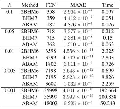
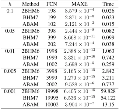
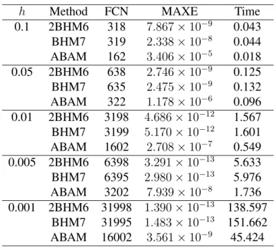
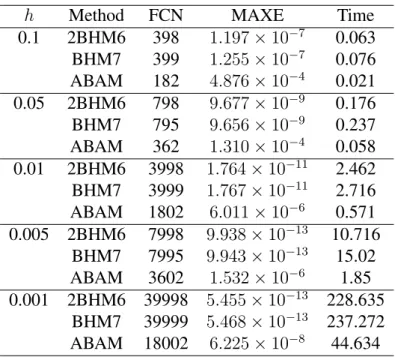
4 RESULTS AND DISCUSSION 46

4.1 Introduction 46

4.2 Implementation in Constant Step Size 47

4.2.1 Discussion I 55

4.3 Implementation in Variable Step Size 56

4.3.1 Discussion II 63

4.4 Compare and Contrast 64

4.4.1 Discussion III 69

4.5 Conclusion 70

4.6 Future Research 70

(9)

REFERENCES 73

(10)

LIST OF TABLES

Table 3.1: Divided Differences 9

Table 4.1: Numerical results for Problem 1. 48

(11)

LIST OF FIGURES

Figure 1.1: Block Method 3

Figure 1.2: Block Hybrid Method 3

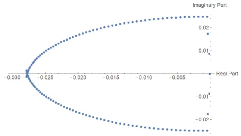
Figure 3.1: Q-Stability area of explicit 2 step block-hybrid method (3.3.2), (3.3.4), (3.3.6), and (3.3.8) of order six. 33 Figure 3.2: Q-Stability area of implicit 2 step block-hybrid method (3.3.12),

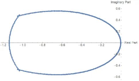
(3.3.14), (3.3.16), and (3.3.19) of order six. 35 Figure 3.3: Q-Stability area of explicit 1 step block-hybrid method (3.3.9)

and (3.3.10) of order seven. 37

Figure 3.4: Q-Stability area of implicit 1 step block-hybrid method (3.3.20)

and (3.3.21) of order seven. 39

Figure 4.1: Maximum error (log10) versus step size for Problem 1. 50 Figure 4.2: Maximum error (log10) versus step size for Problem 2 51 Figure 4.3: Maximum error (log10) versus step size for Problem 3. 51 Figure 4.4: Maximum error (log10) versus step size for Problem 4. 52 Figure 4.5: Maximum error (log10) versus step size for Problem 5. 52 Figure 4.6: Maximum error (log10) versus time taken for Problem 1. 53 Figure 4.7: Maximum error (log10) versus time taken for Problem 2 53 Figure 4.8: Maximum error (log10) versus time taken for Problem 3. 54 Figure 4.9: Maximum error (log10) versus time taken for Problem 4. 54 Figure 4.10: Maximum error (log10) versus time taken for Problem 5. 55 Figure 4.11: Maximum error (log10) versus total steps for Problem 1. 61 Figure 4.12: Maximum error (log10) versus total steps for Problem 2 62 Figure 4.13: Maximum error (log10) versus total steps for Problem 3. 62 Figure 4.14: Maximum error (log10) versus total steps for Problem 4. 63 Figure 4.15: Maximum error (log10) versus total steps for Problem 5. 63 Figure 4.16: Maximum error (log10) versus total steps for Problem 2. 68 Figure 4.17: Maximum error (log10) versus total steps for Problem 3. 68 Figure 4.18: Maximum error (log10) versus total steps for Problem 5. 69

(12)

CHAPTER 1

INTRODUCTION

1.1 General Introduction

The differential equation is an equation that consists of the functions and the derivatives that are widely used in manyﬁelds of study today. These equations are used to model some problems interconnected with the rate of change. We need the results of the equations to solve real-life problems. However, not all the problems can be written as a simple differential equation. The ordinary differential equations (ODEs) are more realistic as they consider the calculation of the current state.

ODEs have a general form as follows:

y^�(t) = g(t, y(t)) for α≤t ≤β,

y(t0) = y0. (1.1.1)

ODEs are very limited when they come to some dynamic problems be- cause ODEs depend on the current time only. Therefore, Delay Differential Equations (DDEs) are another type of differential equation that are more pre- cise on this kind of problem. DDEs involve the past event in the calculation of the current state. The limitation of ODEs can be overcome by modeling the problem using DDEs. In the actual situation, the delay is always there, and exploration around DDEs becomes essential.

We know that not all differential equations can be solved by analytical methods. So, the numerical solution of DDEs is studied in this project. DDEs are the unique type of differential equations whose derivatives at a particular time depend on the preceding time. DDEs can be further divided into two types, which are Retarded Delay Differential Equations (RDDEs) and Neutral Delay Differential Equations (NDDEs). Both RDDEs and NDDEs involve the function and the delay solution, but the only difference is NDDEs have one more term, theﬁrst derivative of the delay term.

(13)

The general form of RDDEs and NDDEs are deﬁned as follows:

RDDEs:

y^�(t) =g(t, y(t), y(t−τ)) , α≤t≤β,

y(t) =ω(t) , t <α; (1.1.2)

NDDEs:

y^�(t) = g(t, y(t), y(t−τ), y^�(t−τ)) , α≤t ≤β,

y(t) = ω(t) , t <α; (1.1.3)

where

τ is the delay,

t−τ is the previous time, y(t−τ) is the delay solution, and ω(t) is an initial function.

There are three types of delay terms in DDEs as follows:

• Constant Delay

y^�(t) = g(t, y(t), y(t−τ)) , y(t)∈R, (1.1.4) whereτ >0and is a constant.

• Time Dependent Delay

y^�(t) = g(t, y(t)y(t−τ(t))) , y(t)∈R, (1.1.5) whereτ(t)>0and is a function that depends ont.

• State Dependent Delay

y^�(t) =g(t, y(t), y(t−τ(t−y(t)))) , y(t)∈R, (1.1.6) whereτ(t−y(t))>0and is a function that depends ontandy(t).

(14)

1.2 Multistep Method

The multistep method is one of the techniques used to solve DDEs. It uses previous points as a reference to approximate the valuey at the targeted point, yn+1. The block method uses the main points as reference points. The step size between all the main points is h. Figure 1.1 shows the relationship between reference points and the targeted point by the step size.

The general form of Block Method is deﬁned as follows:

yn+1 =g(yn, yn−1, yn−2, ...) (1.2.1)

Figure 1.1: Block Method

The block-hybrid method is different from the block method as the main and off-step points will be used together as reference points. The off-step points are the points half step, ^h₂ from the main points. Both the value ofyat the main and off step targeted points can be approximate together by this method. Figure 1.2 shows the relationship between reference points and the targeted point by half the step size.

The general form of Block Hybrid Method is deﬁned as follows:

y_n+¹

2 =g�

yn, y_n₋¹

2, yn−1, y_n₋³

2, yn−2, ...� yn+1 =g�

yn, y_n₋¹

2, yn−1, y_n₋³

2, yn−2, ...� (1.2.2)

Figure 1.2: Block Hybrid Method

(15)

1.3 Importance of Study

DDEs are commonly found in engineering and science studies. Salpeter and Salpeter (1998) estimated the reproductive number and the infection using DDEs Model for epidemiology data on tuberculosis. Makroglou et al. (2006) used DDEs to model the glucose-insulin regulatory system to treat diabetes. It provided a possible mechanism in the secretion of pancreatic insulin. Kajiwara et al. (2012) also used DDEs to construct Lyapunov functional in virology and epidemiology. Gopalsamy (2013) investigated the application of DDEs on pop- ulation dynamics by looking at stability and oscillations.

1.4 Problem Statement

Various mathematical methods have been derived to solve DDEs today. How- ever, not all types of equations can be solved by the analytical method. As such, the numerical method comes in to solve the unsolvable parts. The block method thatfinds the approximation at a few main points concurrently is commonly used to solve ODEs. However, these methods might not get a good approximation when facing the delay term in DDEs. In this study, the block-hybrid method will use information from the main and off-step points to estimate the delay solution to obtain a more refined approximation of the targeted point. Implementation in constant step size requires many iterations when considering a smaller step size to get a more minor accumulated error. The higher number of iterations causes the computation time to become longer. Variable step size is implemented to minimize the total steps or have a more efficient way to solve the problems with minor errors.

(16)

1.5 Aim and Objectives

The objectives of this research are to:

(i) Derive a new block-hybrid method based on the divided difference formula to solve RDDEs. New predictor and corrector equations will be derived as the explicit method and implicit method, respectively.

(ii) Ensure the stability of the new method.

(iii) Implement the new method in variable step size. The step size of the targeted point depends on the local truncation error of the reference points so that the step size can be varied depending on the curve of the equations to minimize the total steps.

(iv) Analyze the accuracy and effectiveness of the new method with a set of speciﬁc tolerances. The analysis is carried out in a few aspects like the number of successful steps/total steps (TS), number of failure steps (FS), number of function evaluations (FCN), the maximum error of absolute value between the com- puted solution and exact solution, and the time for the algorithm.

(17)

1.6 Scope of Study

The primary focus of this study will be on Retarded Delay Differential Equa- tions:

y^�(t) =g(t, y(t), y(t−τ)) , α≤t≤β,

y(t) =ω(t) , t <α; (1.6.1)

where

τ is the delay,

t−τ is the previous time, y(t−τ) is the delay solution, and ω(t) is an initial function.

A new block-hybrid method is used to approximate the numerical solutions of RDDEs. This method is used in predictor-corrector (PECE) mode, with the explicit equation serving as the predictor and the implicit equation serving as the corrector. The step size is varied in every iteration depends on the local truncation error. Three types of delay terms will be used to show how the new method compares to the existing method in terms of accuracy and efﬁciency.

(18)

CHAPTER 2

LITERATURE REVIEW

2.1 Introduction

There are several numerical methods implemented to solve the DDEs. Runge- Kutta method is a popular method used to solve ODEs and can be extended to DDEs. However, it has its limitation when confronting the delay term. So, some research had been carried out by modifying the existing method or implement- ing a new method to ﬁght this delay term. Xie (1992) said the stability and uniqueness of slow oscillate solution would inﬂuence most in solving DDEs.

Continuous Runge-Kutta Methods was proposed in Enright and Hayashi (1997) to solve RDDEs and NDDEs. An iterative system by extrapolation is used as a new idea to handle the vanish delays. This idea is further evaluated in Xu et al. (2010) by using Exponential Runge-Kutta Methods. In Zhang and Chen (2010), it is proved that the Block Boundary Value Methods is convergent of an order under the classical Lipschitz condition.

El-Morshedy and Ruiz-Herrera (2017) proposed a new method using a scalar function to lead the nonlinear terms in the system to obtain the delay- dependent results to cover almost all the delay-independent conditions. Hu and Xiao (2018) study the delay-dependent for a class of nonlinear NDDEs and derived it by generalized Halanay’s inequality. Jamilla et al. (2020) used the LambertWfunction to solve NDDEs which function is deﬁned asW(a)e^W(a)− a= 0. These are some of the parts that the effort being studied to handle DDEs.

(19)

2.2 Block Method

Look closer to the research related to the block method, Hue et al. (2011) proposed the Variable Order Coupled Block Method as the numerical results for DDEs. It used the 2 point 2 step block method of order 5 and 3 point 2 step block method of order 6 to solve DDEs. Majid et al. (2013) derived a 5 point 1 step block method constructed by the divided difference of Newton backward to solve DDEs. Aziz and Majid (2013) modiﬁed the 2 Points Block Method by computing the numerical solution of 2 points simultaneously to produce 2 new equal spaced solutions within the block. This method is based on the pair of implicit and explicit Adams formulas and implemented in predictor-corrector mode. Newton divided difference is derived for interpolation of the delay solutions. In the following year, Aziz et al. (2014) modiﬁed its explicit and implicit methods by recalculating the predictor and corrector formula depends on the step size changed. Yashkun and Aziz (2020) used the new two point Adams predictor-corrector block method derived by the divided difference of Newton to solve NDDEs. The neutral delay is approximated with the technique of cen- tral divided difference.

2.3 Block Hybrid Method

For the block hybrid method, Yap and Ismail (2015) proposed a method of order 3 in predictor-corrector mode to solve DDEs. The method is improved by using the order 6 block hybrid method in Yap et al. (2020). Ismail et al. (2020) derived the block hybrid method based on the Taylor series to solve NDDEs.

2.4 Variable Step Size

Variable step size strategy had been widely used in many research to solve the DDEs. Hue et al. (2011) implemented the strategy in its variable coupled block method. It varies the step size by choosing the maximum step size on the next block. Aziz and Majid (2013) also used this strategy in its modiﬁed 2 point block method. It extended its method by using the Runge-Kutta Fehlberg step size as the strategy to improve the results.

(20)

CHAPTER 3

RESEARCH METHODOLOGY

To derive a new block-hybrid method, both off step and main points are required to proceed with calculation. To implement it in predictor-corrector mode, at least a pair of explicit and implicit methods is needed.

3.1 Divided Difference

The block-hybrid method is constructed based on the divided differences, which are the recursive division process.

Table 3.1: Divided Differences

t f(t) First Divided

Differences Second Divided Differences t0 f[t0]

f� t0, t¹

2

�

=

f

� t1

2

�

−f[t0] t1

2−t0

t¹

2 f�

t¹

2

� f�

t₀, t¹

2, t₁�

= ^f

� t1

2,t1

�

−f

� t0,t1

2

� t1−t0

f� t¹

2, t₁�

= ^f[t¹^]⁻^f

� t1

2

�

t1−t1 2

t1 f[t1] f�

t¹

2, t1, t³

2

� = ^f

� t1,t3

2

�

−f

� t1

2,t1

�

t3 2−t1

2

f� t1, t³

2

�= ^f

� t3

2

�

−f[t1] t3

2−t1

t³

2 f�

t³

2

�

f� t1, t³

2, t2

�

=

f

� t3

2,t2

�

−f

� t1,t3

2

� t2−t1

f� t³

2, t2

�

=

f[t2]−f

� t3

2

�

t2−t3 2

t₂ f[t₂] f�

t³

2, t₂, t⁵

2

� = ^f

� t2,t5

2

�

−f

� t3

2,t2

�

t5 2−t3

2

f� t2, t⁵

2

�= ^f

� t5

2

�

−f[t2] t5

2−t2

t⁵

2 f�

t⁵

2

�

(21)

Then^thdivided differences have a general form as follows:

f� t₀, t¹

2, t₁, ..., t_n−1, t_n₋¹

2, t_n�

= f�

t¹

2, t₁, ..., t_n−1, t_n₋¹

2, t_n�

−f� t0, t¹

2, t1, ..., tn−1, t_n−¹

2

� tn−t0

(3.1.1) Then a list of divided differences is calculated and will be used later.

f[tk] =fk

f� t_k₋¹

2, tk

�= f[tk]−f� t_k₋¹

2

� t_k−t_k₋¹

2

= fk−f_k₋¹

2

h 2

= 2 h

�f_k−f_k₋¹

2

�

f�

tk−1, t_k−¹

2, tk

�

= f�

t_k₋¹

2, tk

�−f�

tk−1, t_k₋¹

2

� tk−tk−1

=

2 h

�

fk−f_k−¹

2

�− ²_h� f_k−¹

2 −f_k−1� h

= 2 h²

�fk−2f_k₋¹

2 +fk−1

�

f� t_k₋³

2, t_k−1, t_k₋¹

2, tk

�

= f�

tk−1, t_k−¹

2, tk

�−f� t_k−³

2, tk−1, t_k−¹

2

� tk−t_k−³

2

=

2 h²

�

fk−2f_k−¹

2 +f_k−1�

− _h²² � f_k₋¹

2 −2fk−1 +f_k₋³

2

�

3 2h

= 4 3h³

�fk−3f_k₋¹

2 + 3fk−1−f_k₋³

2

�

f�

tk−2, t_k−³

2, tk−1, t_k−¹

2, tk

�

= f�

t_k−³

2, tk−1, t_k−¹

2, tk

�

−f�

tk−2, t_k₋³

2, tk−1, t_k₋¹

2

� tk−tk−2

=

4 3h³

�

fk−3f_k−¹

2 + 3f_k−1−f_k−³

2

�

− _3h⁴³ � f_k₋¹

2 −3fk−1+ 3f_k₋³

2 −fk−2

� 2h

= 2 3h⁴

�

fk−4f_k−¹

2 + 6f_k−1−4f_k−³

2 +f_k−2�

(22)

f� t_k₋⁵

2, tk−2, t_k₋³

2, tk−1, t_k₋¹

2, tk

�

= f�

t_k−2, t_k₋³

2, t_k−1, t_k₋¹

2, t_k�

−f� t_k₋⁵

2, t_k−2, t_k₋³

2, t_k−1, t_k₋¹

2

� tk−t_k₋⁵

2

=

2 3h⁴

�fk−4f_k₋¹

2 + 6fk−1−4f_k₋³

2 +fk−2

�

− _3h²⁴ � f_k₋¹

2 −4f_k−1+ 6f_k₋³

2 −4f_k−2+f_k₋⁵

2

�

5 2h

= 4 15h⁵

�

fk−5f_k−¹

2 + 10fk−1−10f_k−³

2 + 5fk−2−f_k−⁵

2

�

f�

tk−3, t_k−⁵

2, tk−2, t_k−³

2, tk−1, t_k−¹

2, tk

�

= f�

t_k₋⁵

2, tk−2, t_k₋³

2, tk−1, t_k₋¹

2, tk

�−f�

tk−3, t_k₋⁵

2, tk−2, t_k₋³

2, tk−1, t_k₋¹

2

� tk−t_k₋⁵

2

=

4 15h⁵

�

fk−5f_k−¹

2 + 10fk−1−10f_k−³

2 + 5fk−2−f_k−⁵

2

�

−_15h⁴⁵ � f_k₋¹

2 −5fk−1+ 10f_k₋³

2 −10fk−2+ 5f_k₋⁵

2 −fk−3

� 3h

= 4 45h⁶

�

fk−6f_k−¹

2 + 15f_k−1−20f_k−³

2 + 15f_k−2−6f_k−⁵

2 +f_k−3� 3.2 Lagrange Interpolation Polynomial

The k^th Lagrange interpolation polynomial, Pk(x), is derived based on the divided differences, where

P_k(t) =f[t_k] +f� t_k₋¹

2, t_k�

(t−t_k) +f�

t_k−1, t_k₋¹

2, t_k�

(t−t_k)�

t−t_k₋¹

2

�

+f� t_k−³

2, tk−1, t_k−¹

2, tk

�

(t−tk)�

t−t_k−¹

2

�

(t−tk−1) +...

+f� t0, t¹

2, t1, ..., t_k₋³

2, tk−1, t_k₋¹

2, tk

�(t−tk)...(t−t1)� t−t¹

2

�

(3.2.1) 3.2.1 The Predictor

Set a variables = t−tk

h to measure tin the unit ofh, where it starts att=tk. Then,t=tk+sh.

Pk(t) =Pk(tk+sh)

=f[tk] +shf� t_k₋¹

2, tk

�+s

� s+1

2

� h²f�

tk−1, t_k₋¹

2, tk

�

+s

� s+ 1

2

�

(s+ 1)h³f� t_k₋³

2, tk−1, t_k₋¹

2, tk

�+...

(3.2.2)

(23)

3.2.2 The Corrector Set a variables = t−t_k+¹

2

h , where the starting point is t = t_k+¹

2. Then, t = t_k+¹

2 +sh.

Pk(t) =Pk

� t_k+¹

2 +sh�

=f� t_k+¹

2

�+shf�

tk, t_k+¹

2

�+s

� s+1

2

� h²f�

t_k₋¹

2, tk, t_k+¹

2

�

+s

� s+1

2

�

(s+ 1)h³f�

tk−1, t_k₋¹

2, tk, t_k+¹

2

�+...

(3.2.3)

Set a variable s = t−tk+1

h , where the starting point is t = tk+1. Then, t = t_k+1+sh.

Pk(t) =Pk(tk+1+sh)

=f[tk+1] +shf� t_k+¹

2, tk+1

�+s

� s+ 1

2

� h²f�

tk, t_k+¹

2, tk+1

�

+s

� s+1

2

�

(s+ 1)h³f� t_k₋¹

2, tk, t_k+¹

2, tk+1

�+...

(3.2.4)

Set a variables = t−t_k+³

2

h , where the starting point is t = t_k+³

2. Then, t = t_k+³

2 +sh.

Pk(t) =Pk

�t_k+³

2 +sh�

=f� t_k+³

2

�+shf�

tk+1, t_k+³

2

�+s

� s+1

2

� h²f�

t_k+¹

2, tk+1, t_k+³

2

�

+s

� s+1

2

�

(s+ 1)h³f�

tk, t_k+¹

2, tk+1, t_k+³

2

�+...

(3.2.5)

Set a variable s = t−tk+2

h , where the starting point is t = t_k+2. Then, t = tk+2+sh.

Pk(t) =Pk(tk+2+sh)

=f[t_k+2] +shf� t_k+³

2, t_k+2� +s

� s+1

2

� h²f�

t_k+1, t_k+³

2, t_k+2� +s

� s+1

2

�

(s+ 1)h³f� t_k+¹

2, t_k+1, t_k+³

2, t_k+2� +...

(3.2.6)

(24)

3.3 Block Hybrid Method

The explicit and implicit methods are derived by integrating the Lagrange interpolation polynomial in Section 3.2. The equation of the explicit method will calculate the predicted y, y^p as an initial estimation for the targeted value by using few previous points as the reference points. Then, the implicit method equation will recalculate they^p to correctedy,y^c as theﬁnal estimation for the targeted value by using both the y^p and few previous points as the reference points. Here, the derivation of two new methods will be discussed, which are 2 step block-hybrid method and 1 step block-hybrid method.

3.3.1 Explicit 2 Step Block Hybrid Method First Off Step Point

Set the off step pointt_k+¹

2 = t_k + 1

2h. Integrate both sides of equation (1.1.2) fromtktot_k+¹

2

� t_{k+ 1}

2

t_k

y^�(t)dt=

� t_{k+ 1}

2

t_k

g(t, y(t), y(t−τ))dt

The function g(t, y(t), y(t−τ))is interpolated by the Lagrange interpolation polynomial equation, (3.2.2).

y_k+¹

2 −yk=

� t_{k+ 1}

2

t_k

Pk(t)dt

Use s = t−tk

h , then t = tk + sh, so dt = hds. To adjust the limits of integration, change the limits whent=tk,s= 0and whent=t_k+¹

2,s = ¹₂. y_k+¹

2 −yk =

� ¹₂

0

Pk(tk+sh)h ds y_k+¹

2 =yk+

� ¹₂

0

f[tk] +shf� t_k₋¹

2, tk

�+s

� s+1

2

� h²f�

tk−1, t_k₋¹

2, tk

�

+s

� s+1

2

�

(s+ 1)h³f� t_k₋³

2, t_k−1, t_k₋¹

2, t_k�

+... ds

(3.3.1)

(25)

where

f[tk] =fk

f� t_k₋¹

2, tk

�= 2 h

�fk−f_k₋¹

2

�

f�

tk−1, t_k₋¹

2, tk

�= 2 h²

�fk−2f_k₋¹

2 +fk−1

�

f� t_k₋³

2, tk−1, t_k₋¹

2, tk

�= 4 3h³

�fk−3f_k₋¹

2 + 3fk−1−f_k₋³

2

�

f�

tk−2, t_k₋³

2, tk−1, t_k₋¹

2, tk

�= 2 3h⁴

�

fk−4f_k−¹

2 + 6f_k−1−4f_k−³

2 +f_k−2� f�

t_k−⁵

2, t_k−2, t_k−³

2, t_k−1, t_k−¹

2, tk

�

= 4

15h⁵

�fk−5f_k₋¹

2 +10fk−1−10f_k₋³

2 + 5fk−2−f_k₋⁵

2

�

Then, the explicit formula for theﬁrst off-step point is derived as follows:

y_k+¹

2 =yk+h

�4277

2880fk−2641 960 f_k−¹

2 + 4991

1440f_k−1

−3649 1440f_k−³

2 + 959

960f_k−2− 95 576f_k−⁵

2

� (3.3.2)

First Main Point

Set the main pointtk+1 =tk+h. Integrate both sides of equation (1.1.2) from t_k tot_k+1 � tk+1

tk

y^�(t)dt=

� tk+1

tk

yk+1−yk =

� tk+1

tk

Pk(t)dt

Use s = t−tk

h , then t = tk + sh, so dt = hds. To adjust the limits of integration, change the limits whent=tk,s= 0and whent=tk+1,s= 1.

(26)

y_k+1−y_k =

� 1 0

P_k(t_k+sh)h ds yk+1 =yk+

� 1 0

2, tk

�+s

� s+ 1

2

� h²f�

tk−1, t_k₋¹

2, tk

�

+s

� s+1

2

�

(s+ 1)h³f� t_k₋³

2, tk−1, t_k₋¹

2, tk

�+... ds

(3.3.3) where

f[tk] =fk

f� t_k₋¹

2, t_k�

= 2 h

�f_k−f_k₋¹

2

�

f�

t_k−1, t_k₋¹

2, t_k�

= 2 h²

�f_k−2f_k₋¹

2 +f_k−1� f�

t_k₋³

2, t_k−1, t_k₋¹

2, t_k�

= 4 3h³

�f_k−3f_k₋¹

2 + 3f_k−1−f_k₋³

2

�

f�

t_k−2, t_k₋³

2, t_k−1, t_k₋¹

2, t_k�

= 2 3h⁴

�

fk−4f_k−¹

2 + 6fk−1−4f_k−³

2 +fk−2

�

f� t_k−⁵

2, tk−2, t_k−³

2, tk−1, t_k−¹

2, tk

�

= 4

15h⁵

�fk−5f_k₋¹

2 +10fk−1−10f_k₋³

2 + 5fk−2−f_k₋⁵

2

�

Then, the explicit formula for theﬁrst main point is derived as follows:

yk+1 =yk+h

�344

45fk−3881 180 f_k−¹

2 +919

30 fk−1

−2143 90 f_k−³

2 +877

90 fk−2− 33 20f_k−⁵

2

� (3.3.4)

Second Off Step Point Set the off step pointt_k+³

2 = tk + 3

2h. Integrate both sides of equation (1.1.2) fromtktot_k+³

2

� t_{k+ 3}

2

tk

y^�(t)dt=

� t_{k+ 3}

2

tk

The function g(t, y(t), y(t−τ))is interpolated by the Lagrange interpolation

(27)

polynomial equation, (3.2.2).

y_k+³

2 −yk=

� t_{k+ 3}

2

tk

Pk(t)dt

Use s = t−tk

h , then t = tk + sh, so dt = hds. To adjust the limits of integration, change the limits whent=tk,s= 0and whent=t_k+³

2,s = ³₂. y_k+³

2 −yk =

� ³₂

0

Pk(tk+sh)h ds y_k+³

2 =y_k+

� ³₂

0

f[t_k] +shf� t_k₋¹

2, t_k� +s

� s+1

2

� h²f�

t_k−1, t_k₋¹

2, t_k� +s

� s+1

2

�

(s+ 1)h³f� t_k₋³

2, t_k−1, t_k₋¹

2, t_k�

+... ds

(3.3.5) where

f[t_k] =f_k f�

t_k−¹

2, tk

�= 2 h

�fk−f_k−¹

2

�

f�

tk−1, t_k−¹

2, tk

�

= 2 h²

�

fk−2f_k−¹

2 +fk−1

�

f� t_k−³

2, tk−1, t_k−¹

2, tk

�

= 4 3h³

�

fk−3f_k−¹

2 + 3fk−1−f_k−³

2

�

f�

tk−2, t_k−³

2, tk−1, t_k−¹

2, tk

�

= 2 3h⁴

�fk−4f_k₋¹

2 + 6fk−1−4f_k₋³

2 +fk−2

�

f� t_k₋⁵

2, tk−2, t_k₋³

2, tk−1, t_k₋¹

2, tk

�= 4

15h⁵

�f_k−5f_k₋¹

2 +10f_k−1−10f_k₋³

2 + 5f_k−2−f_k₋⁵

2

�

Then, the explicit formula for the second off-step point is derived as follows:

y_k+³

2 =yk+h

�8253

320 fk− 27771 320 f_k₋¹

2 +21207 160 fk−1

−17193 160 f_k₋³

2 + 14469

320 fk−2− 2499 320 f_k₋⁵

2

� (3.3.6)

Second Main Point

Set the main pointt_k+2 =t_k+ 2h. Integrate both sides of equation (1.1.2) from

(28)

t_k tot_k+2 � tk+2

tk

y^�(t)dt=

� tk+2

tk

yk+2−yk =

� tk+2

tk

Pk(t)dt

Use s = t−tk

h , then t = tk + sh, so dt = hds. To adjust the limits of integration, change the limits whent=tk,s= 0and whent=tk+2,s= 2.

yk+2−yk =

� 2 0

Pk(tk+sh)h ds yk+2 =yk+

� 2 0

2, tk

�+s

� s+ 1

2

� h²f�

tk−1, t_k₋¹

2, tk

�

+s

� s+1

2

�

(s+ 1)h³f� t_k₋³

2, t_k−1, t_k₋¹

2, t_k�

+... ds

(3.3.7) where

f[tk] =fk

f� t_k−¹

2, tk

�

= 2 h

�

fk−f_k−¹

2

�

f�

tk−1, t_k−¹

2, tk

�

= 2 h²

�

fk−2f_k−¹

2 +fk−1

�

f� t_k−³

2, tk−1, t_k−¹

2, tk

�

= 4 3h³

�

fk−3f_k−¹

2 + 3fk−1−f_k−³

2

�

f�

tk−2, t_k−³

2, tk−1, t_k−¹

2, tk

�

= 2 3h⁴

�fk−4f_k₋¹

2 + 6fk−1−4f_k₋³

2 +fk−2

�

f� t_k₋⁵

2, tk−2, t_k₋³

2, tk−1, t_k₋¹

2, tk

�= 4

15h⁵

�f_k−5f_k₋¹

2 +10f_k−1−10f_k₋³

2 + 5f_k−2−f_k₋⁵

2

�

Then, the explicit formula for the second main point is derived as follows:

yk+2 =yk+h

�625

9 fk− 3856 15 f_k₋¹

2 + 18532 45 fk−1

−15488 45 f_k₋³

2 + 2219

15 fk−2− 1168 45 f_k₋⁵

2

� (3.3.8)

(29)

3.3.2 Explicit 1 Step Block Hybrid Method Evaluate equations (3.3.1) and (3.3.7) up to the term

f�

tk−3, t_k−⁵

2, tk−2, t_k−³

2, tk−1, t_k−¹

2, tk

�= 4

45h⁶

�fk−6f_k₋¹

2 + 15fk−1 −20f_k₋³

2 + 15fk−2−6f_k₋⁵

2 +fk−3

�.

Off Step Point

The explicit formula for off-step point is derived as follows:

y_k+¹

2 =yk+h

�198721

120960fk− 18637 5040 f_k₋¹

2 + 235183

40320 fk−1− 5377 945 f_k₋³

2

+135713

40320 fk−2− 5603 5040f_k₋⁵

2 + 19087 120960fk−3

�

(3.3.9) Main Point

The explicit formula for the main point is derived as follows:

yk+1 =yk+h

�14281

1512 fk− 2039 63 f_k−¹

2 +145261

2520 f_k−1− 56534 945 f_k−³

2

+92621

2520 f_k−2 −3923 315 f_k−⁵

2 + 13613 7560 f_k−3

�

(3.3.10)