Digital signal processing (DSP) is concerned with the representation of signals as a sequence of numbers and the algorithmic operations carried out on the signals to extract specific information contained in them. In barely 40 years the field of digital signal processing has matured considerably due to the phenomenal growth in both research and applications, and almost every university is now offering at least one or more courses at the upper division and/or first-year graduate level on this subject. With the increasing availability of powerful personal computers and workstations at affordable prices, it has become easier to provide the student with a practical environment to verify the concepts and the algorithms learned in a lecture course.

This book is for a computer-based DSP laboratory course that supplements a lecture course on the subject. It includes 11 laboratory exercises with each exercise containing a number of projects to be carried out on a computer. The total number of projects may be more than what can be completed in a quarter- or a semester-long course assuming a three-hour per week laboratory. It is suggested that the instructor select pertinent projects that are more relevant to the lecture course he/she is teaching. If the computer laboratory is open for longer hours, it is recommended that the student be encouraged to come to the laboratory for longer periods of time to enable him/her to complete all projects.

The programming language used in this book is MATLAB,¹widely used for high-perfor- mance numerical computation and visualization. The book assumes that the reader has no background in MATLAB and teaches him/her through tested programs in the first half of the book the basics of this powerful language in solving important problems in signal processing.

In the second half of the book the student is asked to write the necessary MATLAB programs to carry out the projects. I believe students learn the intricacies of problem solving with MATLAB faster by using tested, complete programs and later writing simple programs to solve specific problems. A short review of the key concepts and features of MATLAB is provided in Appendix A.

Altogether there are 75 MATLAB programs in the text that have been tested under version 7.0 of MATLAB and version 6.3 of the Signal Processing Toolbox. The programs listed in this book are not necessarily the fastest with regard to their execution speeds, nor are they the shortest. They have been written for maximum clarity without detailed explanations.

This book includes a CD containing all MATLAB programs for the PC running Windows

1MATLAB is a registered trademark of The Mathworks, Inc., 3 Apple Hill Dr., Natick, MA 01760, phone:

508-647-7000,http://www.mathworks.com.

vii

(8)

XP, the /pagebreak Macintosh computers running Mac OS X and UNIX workstations. All programs are also available from the Internet siteftp://iplserv.ece.ucsb.eduin the directory /pub/mitra/Labs.

Each laboratory exercise contains a number of projects for the students to implement on their computers. Each project is followed by a series of questions the students must answer before embarking on the following project. These questions are designed to teach the student the fundamentals of MATLAB and also the key concepts of DSP. For the latter part, each exercise includes a section summarizing the materials necessary for a quick review of DSP materials necessary to carry out the projects included in the exercise. For further details and explanations, each exercise includes at the end a list of DSP texts with specific chapter and/or section numbers. Each exercise also includes a section summarizing the MATLAB commands used to enable the student to find out more about one or more of these commands, if necessary, through thehelpcommand. A brief explanation of all MATLAB functions used in this book is given in Appendix B.

A novel feature of this book contains is the inclusion of partially written report documents for each of the first 10 laboratory exercises in the CD provided. These reports are written in Microsoft Word. The students fill in the space provided for answers to the questions as they proceed through the projects. This feature permits the students to complete more work in a specified amount of time than would have been possible without it. The answers of the students should appear in a different font to make it easier for the laboratory instructor to evaluate the student’s work. The completed report also can serve as a guide for writing reports in other laboratory courses.

This book has evolved from teaching a laboratory component to an upper-division course on digital signal processing at the University of California, Santa Barbara, for the last 10 years. I thank my former students Drs. Stefan Thurnhofer and Ing-Song Lin for their assistance in developing the preliminary version of the laboratory course materials. I also thank the students who took the upper division course and provided valuable comments that have improved the contents and style of the laboratory portion of the course. The complete manuscript of this book has been reviewed by Professor Hrvoje Babic of the University of Zagreb, Zagreb, Croatia; Professor Tamal Bose of the Utah State University, Logan, Utah; Professor Ulrich Heute of the University of Kiel, Kiel, Germany; Professor Ottar Johnsen of the Ecole d’Ing´enieurs de Friboug, Friboug, Switzerland; Professor Abul N.

Khondker of the Clarkson University, Potsdam, New York; Professor V. John Mathews of the University of Utah, Salt Lake City, Utah and Professor Yao Wang of the Polytechnic University, Brooklyn, New York. I thank them for their valuable comments. I thank my former students, Drs. Rajeev Gandhi, Michael Moore and Debargha Mukherjee, for their assistance in proofreading the manuscript and checking all the programs included in the first version of this book. I also thank my students John Berger and Yang Zhang for updating all programs in the present version. I acknowledge with gratitude the support of the Office of Instructional Development at the University of California, Santa Barbara, for providing me with two instructional improvement grants to develop the laboratory course. Finally, I thank my son Goutam for the cover design of my book.

Every attempt has been made to ensure the accuracy of all materials in this book, including the MATLAB programs. I would, however, appreciate readers bringing to my attention any

(9)

ix

errors that may have appeared in the printed version for reasons beyond my control and that of the publisher. These errors and any other comments can be communicated to me by e-mail addressed to: [email protected].

Santa Barbara Sanjit K. Mitra

(10)

(11)

Discrete-Time Signals

in the Time Domain 1

1.1 Introduction

Digital signal processing is concerned with the processing of a discrete-time signal, called the input signal, to develop another discrete-time signal, called the output signal, with more desirable properties. In certain applications, it may be necessary to extract some key properties of the original signal using specific digital signal processing algorithms. It is also possible to investigate the properties of a discrete-time system by observing the output signals for specific input signals. It is thus important to learn first how to generate in the time domain some basic discrete-time signals in MATLAB and perform elementary operations on them, which are the main objectives of this first exercise. A secondary objective is to learn the application of some basic MATLAB commands and how to apply them in simple digital signal processing problems.

1.2 Getting Started

The CD provided with this book contains all of the MATLAB programs and the partially written reports for both the PC and the Macintosh computers. In particular, it includes both PC and Macintosh versions of the MATLAB M-files of the first 10 exercises in folders grouped by chapters and report documents written in Microsoft Word in folders also grouped by chapters. After the completion of a project of a laboratory exercise, you record in the report of that exercise the answers to questions referring to this project at their designated locations.

Installation Instructions for a PC

To copy the program and the report folders onto the hard disk of a PC running Windows XP follow the steps given below:

1. Insert the CD.

2. Open theMy Computerwindow by double-clicking on its icon displayed on the Desktop.

3. Open the window of the CD by double-clicking on its icon.

4. Open the window of the desired hard drive by double-clicking on its icon. Depend- ing on your setup, it may be necessary to open another window by double-clicking

1

(12)

onMy Computericon before you can select the destination hard drive.

5. In the CD drive window, select the folder markedPCand drag it to the directory displayed in the hard drive window where you would like to copy the files.

Installation Instructions for a Macintosh computer

To copy the program and the report folders on the hard disk of a Macintosh computer running Mac OS X follow the steps given below:

1. Insert the CD.

2. Open the hard drive window by double-clicking on its icon displayed on the Desk- top.

3. Open the window of the CD by double-clicking on its icon.

4. In the CD window, select the folder markedMACand drag it to the directory displayed in the hard drive window where you would like to copy the files.

Downloading from the World Wide Web

The web site for downloading the files to a computer ishttp://iplserv.ece.ucsb.edu. The directories containing the files for the PC, Macintosh computer, and UNIX workstation are as follows:

pub/mitra/Labs/pc pub/mitra/Labs/mac

pub/mitra/Labs/unix(M-files only)

To download the files from this site to your computer, follow the steps given below:

1. Open the available Internet web browser.

2. Typehttp://iplserv.ece.ucsb.eduin the URL window.

3. Double-click on the desired directory (the directory for the PC and Macintosh versions are shown above).

4. Double-click on the desired file for downloading. You will get a dialog box asking where you would like to save the file.

1.3 Background Review

R1.1 A discrete-time signal is represented as a sequence of numbers, calledsamples. A sample value of a typical discrete-time signal or sequence{x[n]}is denoted asx[n]with the argumentnbeing an integer in the range−∞and∞. For convenience, the sequence {x[n]}is often denoted without the curly brackets.

(13)

1.3 Background Review

3

R1.2 The discrete-time signal may be a finite length or an infinite length sequence. A finite length (also calledfinite durationorfinite extent) sequence is defined only for a finite time interval:

N₁≤n≤N₂, (1.1)

where−∞< N₁andN₂ <∞withN₂ ≥ N₁. The length or durationN of the finite length sequence is

N =N₂−N₁+ 1. (1.2)

R1.3 A sequencex[n]˜ satisfying

˜

x[n] = ˜x[n+kN] for all n, (1.3) is called aperiodic sequencewith a periodN whereN is a positive integer andkis any integer.

R1.4 Theenergyof a sequencex[n]is defined by E=

∞ n=−∞

|x[n]|². (1.4)

The energy of a sequence over a finite interval−K≤n≤Kis defined by EK =

K n=−K

|x[n]|². (1.5)

R1.5 Theaverage powerof an aperiodic sequencex[n]is defined by Pav = lim

K→∞

1

2K+ 1EK = lim

K→∞

1 2K+ 1

K n=−K

|x[n]|². (1.6)

The average power of a periodic sequencex[n]˜ with a periodN is given by Pav = 1

N

N−1 n=0

|x[n]˜ |². (1.7)

R1.6 Theunit sample sequence, often called thediscrete-time impulseor theunit impulse, denoted byδ[n], is defined by

δ[n] =

1, forn= 0,

0, forn= 0. (1.8)

Theunit step sequence, denoted byµ[n], is defined by µ[n] =

1, forn≥0,

0, forn <0. (1.9)

(14)

R1.7 Theexponential sequenceis given by

x[n] =Aαⁿ, (1.10)

whereAandαare real or complex numbers. By expressing α=e⁽^σ^o⁺^jω^o⁾, and A=|A|e^jφ, we can rewrite Eq. (1.10) as

x[n] =|A|e^σôⁿ⁺^j⁽^ωôⁿ⁺^φ⁾=|A|e^σôⁿcos(ω_on+φ) +j|A|e^σôⁿsin(ω_on+φ). (1.11) R1.8 Thereal sinusoidal sequencewith a constant amplitude is of the form

x[n] =Acos(ωon+φ), (1.12) whereA,ω_o, andφare real numbers. The parametersA,ω_o, andφin Eqs. (1.11) and (1.12) are called, respectively, theamplitude, theangular frequency, and theinitial phase of the sinusoidal sequencex[n]. f_o=ω_o/2πis thefrequency.

R1.9 The complex exponential sequence of Eq. (1.11) withσo = 0and the sinusoidal sequence of Eq. (1.12) are periodic sequences ifωoNis an integer multiple of2π, that is,

ωoN = 2πr, (1.13)

whereN is a positive integer andris any integer. The smallest possibleN satisfying this condition is theperiodof the sequence.

R1.10 Theproductof two sequencesx[n]andh[n]of lengthN yields a sequencey[n], also of lengthN, as given by

y[n] =x[n]·h[n]. (1.14)

Theadditionof two sequencesx[n]andh[n]of lengthN yields a sequencey[n], also of lengthN, as given by

y[n] =x[n] +h[n]. (1.15)

Themultiplicationof a sequencex[n]of lengthNby a scalarAresults in a sequencey[n]

of lengthNas given by

y[n] =A·x[n]. (1.16)

Thetime-reversalof a sequencex[n]of infinite length results in a sequencey[n]of infinite length as defined by

y[n] =x[−n]. (1.17)

Thedelayof a sequencex[n]of infinite length by a positive integerMresults in a sequence y[n]of infinite length given by

y[n] =x[n−M]. (1.18)

IfMis a negative integer, the operation indicated in Eq. (1.18) results in anadvanceof the sequencex[n].

A sequence x[n] of length N can be appended by another sequence g[n] of length M resulting in a longer sequencey[n]of lengthN+M given by

{y[n]}={{x[n]},{g[n]}}. (1.19)

(15)

1.4 MATLAB Commands Used

5

1.4 MATLAB Commands Used

The MATLAB commands you will encounter in this exercise are as follows:

Operators and Special Characters

: . + - * / ;

%

Elementary Matrices and Matrix Manipulation

i ones pi rand randn zeros

Elementary Functions

cos exp imag real

Data Analysis sum

Two-Dimensional Graphics

axis grid legend plot stairs

stem title xlabel ylabel

General Purpose Graphics Functions

clf subplot

Signal Processing Toolbox sawtooth square

For additional information on these commands, see theMATLAB Reference Guide[Mat05]

or typehelp commandnamein the Command window. A brief explanation of the MATLAB functions used here can be found in Appendix B.

1.5 Generation of Sequences

The purpose of this section is to familiarize you with the basic commands in MATLAB for signal generation and for plotting the generated signal. MATLAB has been designed to operate on data stored as vectors or matrices. For our purposes, sequences will be stored as vectors. Therefore, all signals are limited to being causal and of finite length . The steps to follow to execute the programs listed in this book depend on the platform being used to run the MATLAB.

(16)

MATLAB on the Windows PC

The program can be executed by typing the name of the program without.min the Command window and hitting the carriage return. Alternately, chooseOpen from theFile menu in the Command window and choose the desired M-file. This opens the M-file in the Editor/Debugger window in which an M-file can be executed using the Run command under theToolsmenu.

MATLAB on the Macintosh

The program can be executed by typing the name of the program without.min the Command window and hitting the carriage return. Alternately, it can be copied into the Editor Window by using the Open M-File command on your screen and then choosing theSave and Executecommand on your screen.

Project 1.1 Unit Sample and Unit Step Sequences

Two basic discrete-time sequences are the unit sample sequence and the unit step sequence of Eqs. (1.8) and (1.9), respectively. A unit sample sequenceu[n] of lengthNcan be generated using the MATLAB command

u = [1 zeros(1,N -1)];

A unit sample sequenceud[n]of lengthNand delayed byMsamples, whereM < N, can be generated using the MATLAB command

ud = [zeros(1,M) 1 zeros(1,N - M - 1)];

Likewise, a unit step sequences[n] of lengthN can be generated using the MATLAB command

s = [ones(1,N)];

A delayed unit step sequence can be generated in a manner similar to that used in the generation of a delayed unit sample sequence.

Program P1 1 can be used to generate and plot a unit sample sequence.

% Program P1_1

% Generation of a Unit Sample Sequence clf;

% Generate a vector from -10 to 20 n = -10:20;

% Generate the unit sample sequence u = [zeros(1,10) 1 zeros(1,20)];

% Plot the unit sample sequence stem(n,u);

xlabel(’Time index n’);ylabel(’Amplitude’);

title(’Unit Sample Sequence’);

axis([-10 20 0 1.2]);

(17)

1.5 Generation of Sequences

7

Questions:

Q1.1 Run Program P1 1 to generate the unit sample sequenceu[n]and display it.

Q1.2 What are the purposes of the commandsclf,axis,title,xlabel, andylabel?

Q1.3 Modify Program P1 1 to generate a delayed unit sample sequenceud[n]with a delay of11samples. Run the modified program and display the sequence generated.

Q1.4 Modify Program P1 1 to generate a unit step sequences[n]. Run the modified program and display the sequence generated.

Q1.5 Modify Program P1 1 to generate a delayed unit step sequence sd[n] with an advance of7samples. Run the modified program and display the sequence generated.

Project 1.2 Exponential Signals

Another basic discrete-time sequence is the exponential sequence. Such a sequence can be generated using the MATLAB operators.^andexp.

Program P1 2 given below can be employed to generate a complex-valued exponential sequence.

% Program P1_2

% Generation of a complex exponential sequence clf;

c = -(1/12)+(pi/6)*i;

K = 2;

n = 0:40;

x = K*exp(c*n);

subplot(2,1,1);

stem(n,real(x));

title(’Real part’);

subplot(2,1,2);

stem(n,imag(x));

title(’Imaginary part’);

Program P1 3 given below can be employed to generate a real-valued exponential sequence.

% Program P1_3

% Generation of a real exponential sequence clf;

n = 0:35; a = 1.2; K = 0.2;

x = K*a.^+n;

stem(n,x);

(18)

Questions:

Q1.6 Run Program P1 2 and generate the complex-valued exponential sequence.

Q1.7 Which parameter controls the rate of growth or decay of this sequence? Which parameter controls the amplitude of this sequence?

Q1.8 What will happen if the parametercis changed to(1/12)+(pi/6)*i?

Q1.9 What are the purposes of the operatorsrealandimag?

Q1.10 What is the purpose of the commandsubplot?

Q1.11 Run Program P1 3 and generate the real-valued exponential sequence.

Q1.12 Which parameter controls the rate of growth or decay of this sequence? Which parameter controls the amplitude of this sequence?

Q1.13 What is the difference between the arithmetic operators^and.^?

Q1.14 What will happen if the parameterais less than1? Run Program P1 3 again with the parameterachanged to0.9and the parameterKchanged to20.

Q1.15 What is the length of this sequence and how can it be changed?

Q1.16 You can use the MATLAB commandsum(s.*s)to compute the energy of a real sequences[n] stored as a vectors. Evaluate the energy of the real-valued exponential sequencesx[n]generated in Questions Q1.11 and Q1.14.

Project 1.3 Sinusoidal Sequences

Another very useful class of discrete-time signals is the real sinusoidal sequence of the form of Eq. (1.12). Such sinusoidal sequences can be generated in MATLAB using the trigonometric operatorscosandsin.

Program P1 4 is a simple example that generates a sinusoidal signal.

% Program P1_4

% Generation of a sinusoidal sequence n = 0:40;

f = 0.1;

phase = 0;

A = 1.5;

arg = 2*pi*f*n - phase;

x = A*cos(arg);

clf; % Clear old graph

stem(n,x); % Plot the generated sequence axis([0 40 -2 2]);

grid;

(19)

1.5 Generation of Sequences

9

title(’Sinusoidal Sequence’);

xlabel(’Time index n’);

ylabel(’Amplitude’);

axis;

Questions:

Q1.17 Run Program P1 4 to generate the sinusoidal sequence and display it.

Q1.18 What is the frequency of this sequence and how can it be changed? Which parameter controls the phase of this sequence? Which parameter controls the amplitude of this sequence? What is the period of this sequence?

Q1.19 What is the length of this sequence and how can it be changed?

Q1.20 Compute the average power of the generated sinusoidal sequence.

Q1.21 What are the purposes of theaxisandgridcommands?

Q1.22 Modify Program P1 4 to generate a sinusoidal sequence of frequency 0.9and display it. Compare this new sequence with the one generated in Question Q1.17. Now, modify Program P1 4 to generate a sinusoidal sequence of frequency1.1and display it.

Compare this new sequence with the one generated in Question Q1.17. Comment on your results.

Q1.23 Modify the above program to generate a sinusoidal sequence of length50, fre- quency0.08, amplitude2.5, and phase shift90degrees and display it. What is the period of this sequence?

Q1.24 Replace the stemcommand in Program P1 4 with the plotcommand and run the program again. What is the difference between the new plot and the one generated in Question Q1.17?

Q1.25 Replace thestemcommand in Program P1 4 with thestairscommand and run the program again. What is the difference between the new plot and those generated in Questions Q1.17 and Q1.24?

Project 1.4 Random Signals

A random signal of lengthNwith samples uniformly distributed in the interval(0,1)can be generated by using the MATLAB command

x = rand(1,N);

Likewise, a random signalx[n]of lengthNwith samples normally distributed with zero mean and unity variance can be generated by using the following MATLAB command

x = randn(1,N);

(20)

Questions:

Q1.26 Write a MATLAB program to generate and display a random signal of length100 whose elements are uniformly distributed in the interval[−2,2].

Q1.27 Write a MATLAB program to generate and display a Gaussian random signal of length75whose elements are normally distributed with zero mean and a variance of3.

Q1.28 Write a MATLAB program to generate and display five sample sequences of a random sinusoidal signal of length31

{X[n]}={A·cos(ωon+φ)}, (1.20) where the amplitudeAand the phaseφare statistically independent random variables with uniform probability distribution in the range0≤A≤4for the amplitude and in the range 0≤φ≤2πfor the phase.

1.6 Simple Operations on Sequences

As indicated earlier, the purpose of digital signal processing is to generate a signal with more desirable properties from one or more given discrete-time signals. The processing algorithm consists of performing a combination of basic operations such as addition, scalar multiplication, time-reversal, delaying, and product operation (see R1.10). We consider here three very simple examples to illustrate the application of such operations .

Project 1.5 Signal Smoothing

A common example of a digital signal processing application is the removal of the noise component from a signal corrupted by additive noise. Lets[n]be the signal corrupted by a random noised[n]resulting in the noisy signal x[n] = s[n] +d[n]. The objective is to operate onx[n]to generate a signaly[n]which is a reasonable approximation tos[n].

To this end, a simple approach is to generate an output sample by averaging a number of input samples around the sample at instantn. For example, a three-point moving average algorithm is given by

y[n] =¹₃(x[n−1] +x[n] +x[n+ 1]). (1.21) Program P1 5 implements the above algorithm.

% Program P1_5

% Signal Smoothing by Averaging clf;

R = 51;

d = 0.8*(rand(R,1) - 0.5); % Generate random noise m = 0:R-1;

(21)

1.6 Simple Operations on Sequences

11

s = 2*m.*(0.9.^m); % Generate uncorrupted signal x = s + d’; % Generate noise corrupted signal subplot(2,1,1);

plot(m,d’,’r-’,m,s,’g--’,m,x,’b-.’);

legend(’d[n] ’,’s[n] ’,’x[n] ’);

x1 = [0 0 x];x2 = [0 x 0];x3 = [x 0 0];

y = (x1 + x2 + x3)/3;

subplot(2,1,2);

plot(m,y(2:R+1),’r-’,m,s,’g--’);

legend(’y[n] ’,’s[n] ’);

Questions:

Q1.29 Run Program P1 5 and generate all pertinent signals.

Q1.30 What is the form of the uncorrupted signals[n]? What is the form of the additive noised[n]?

Q1.31 Can you use the statementx = s + dto generate the noise-corrupted signal? If not, why not?

Q1.32 What are the relations between the signalsx1,x2, andx3, and the signalx?

Q1.33 What is the purpose of thelegendcommand?

Project 1.6 Generation of Complex Signals

More complex signals can be generated by performing the basic opertations on simple signals. For example, an amplitude modulated signalcan be generated by modulating a high-frequency sinusoidal signal x_H[n] = cos(ωHn)with a low-frequency modulating signalx_L[n] cos(ωLn). The resulting signaly[n]is of the form

y[n] =A(1 +m·xL[n])xH[n] =A(1 +m·cos(ωLn)) cos(ωHn),

wherem, called themodulation index, is a number chosen to ensure that(1 +m·xL[n]) is positive for alln. Program P1 6 can be used to generate an amplitude modulated signal.

% Program P1_6

% Generation of amplitude modulated sequence clf;

n = 0:100;

m = 0.4;fH = 0.1; fL = 0.01;

xH = sin(2*pi*fH*n);

xL = sin(2*pi*fL*n);

(22)

y = (1+m*xL).*xH;

stem(n,y);grid;

Questions:

Q1.34 Run Program P1 6 and generate the amplitude modulated signaly[n]for various values of the frequencies of the carrier signalxH[n]and the modulating signalxL[n], and various values of the modulation indexm.

Q1.35 What is the difference between the arithmetic operators*and.*?

As the frequency of a sinusoidal signal is the derivative of its phase with respect to time, to generate a swept-frequency sinusoidal signal whose frequency increases linearly with time, the argument of the sinusoidal signal must be a quadratic function of time. Assume that the argument is of the forman²+bn(i.e. the angular frequency is2an+b). Solve for the values ofaandbfrom the given conditions (minimum angular frequency and maximum angular frequency). Program P1 7 is an example program to generate this kind of signal.

% Program P1_7

% Generation of a swept frequency sinusoidal sequence n = 0:100;

a = pi/2/100;

b = 0;

arg = a*n.*n + b*n;

x = cos(arg);

clf;

stem(n, x);

axis([0,100,-1.5,1.5]);

title(’Swept-Frequency Sinusoidal Signal’);

xlabel(’Time index n’);

grid; axis;

Questions:

Q1.36 Run Program P1 7 and generate the swept-frequency sinusoidal sequencex[n].

Q1.37 What are the minimum and maximum frequencies of this signal?

Q1.38 How can you modify the above program to generate a swept sinusoidal signal with a minimum frequency of0.1and a maximum frequency of0.3?

(23)

1.7 Workspace Information

13

1.7 Workspace Information

The commandswhoandwhoscan be used to get information about the variables stored in the workspace and their sizes created in running various MATLAB programs at any time.

Questions:

Q1.39 Typewhoin the Command window. What information is displayed in the Com- mand window as a result of this command?

Q1.40 Typewhosin the Command window. What information is displayed in the Com- mand window as a result of this command?

1.8 Other Types of Signals (Optional)

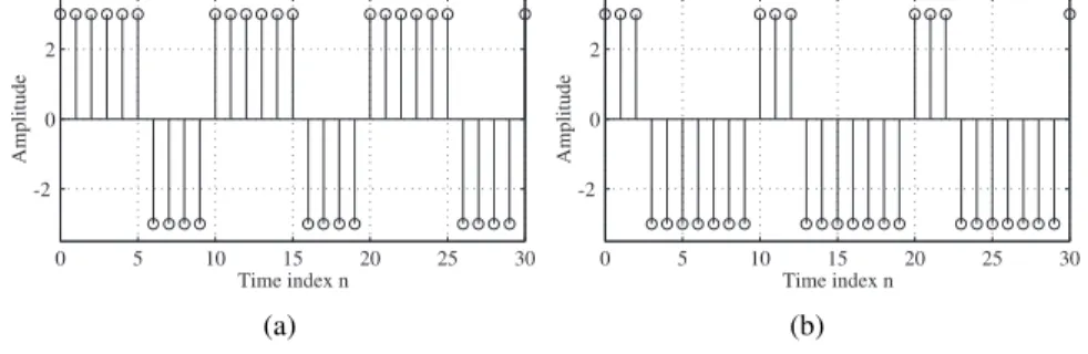
Project 1.7 Square wave and Sawtooth Signals

MATLAB functionssquareandsawtoothcan be used to generate sequences of the types shown in Figures 1.1 and 1.2, respectively.

0 5 10 15 20 25 30

-2 0 2

Time index n

Amplitude

0 5 10 15 20 25 30

-2 0 2

Time index n

Amplitude

(a) (b)

Figure 1.1 Square wave sequences.

Question:

Q1.41 Write MATLAB programs to generate the square wave and the sawtooth wave sequences of the types shown in Figures A.1 and 1.2. Using these programs, generate and plot the sequences.

(24)

0 10 20 30 40 50 -2

-1 0 1 2

Time index n

Amplitude

0 10 20 30 40 50

-2 -1 0 1 2

Time index n

Amplitude

(a) (b)

Figure 1.2 Sawtooth wave sequences.

1.9 Background Reading

[1] E. Cunningham. Digital Filtering: An Introduction. Houghton-Mifflin, Boston MA, 1992. Secs. 1.2–1.3.

[2] D. J. DeFatta, J. G. Lucas, and W. S. Hodgkiss.Digital Signal Processing: A System Design Approach. Wiley, New York NY, 1988. Secs. 2.1.2–2.1.4.

[3] L. B. Jackson. Digital Filters and Signal Processing. Kluwer, Boston MA, third edition, 1996. Secs. 2.2–2.3.

[4] R. Kuc. Introduction to Digital Signal Processing. McGraw-Hill, New York NY, 1988. Secs. 2-2, 2-4.

[5] L. C. Ludeman. Fundamentals of Digital Signal Processing. Harper & Row, New York NY, 1986. Sec. 1.2.

[6] S. K. Mitra.Digital Signal Processing: A Computer-Based Approach. McGraw-Hill, New York NY, third edition, 2005. Secs. 2.1–2.2.

[7] A. V. Oppenheim, R. W. Schafer, and J. R. Buck. Discrete-Time Signal Processing.

Prentice-Hall, Upper Saddle River NJ, second edition, 1998. Sec. 2.1.

[8] B. Porat. A Course in Digital Signal Processing. Wiley, New York NY, 1996. Secs.

2.7–2.8.

[9] J. G. Proakis and D. G. Manolakis.Digital Signal Processing: Principles, Algorithms, and Applications. Prentice-Hall, Upper Saddle River NJ, third edition, 1996. Secs.

2.2–2.4.

[10] R. A. Roberts and C. T. Mullis.Digital Signal Processing, Addison-Wesley. Reading MA, 1987. Sec. 2.2.

(25)

Discrete-Time Systems

in the Time Domain 2

2.1 Introduction

A discrete-time system processes an input signal in the time-domain to generate an output signal with more desirable properties by applying an algorithm composed of simple operations on the input signal and its delayed versions. The aim of this second exercise is to illustrate the simulation of some simple discrete-time systems on the computer using MATLAB and investigate their time domain properties.

2.2 Background Review

R2.1 For alineardiscrete-time system , ify₁[n]andy₂[n]are the responses to the input sequencesx₁[n]andx₂[n], respectively, then for an input

x[n] =α x₁[n] +β x₂[n], (2.1) the response is given by

y[n] =α y₁[n] +β y₂[n]. (2.2) The superposition property of Eq. (2.2) must hold for any arbitrary constantsαandβand for all possible inputsx₁[n]andx₂[n]. If Eq. (2.2) does not hold for at least one set of nonzero values ofαandβ, or one set of nonzero input sequencesx₁[n]andx₂[n], then the system isnonlinear.

R2.2 For atime-invariantdiscrete-time system , ify₁[n]is the response to an inputx₁[n], then the response to an input

x[n] =x₁[n−n_o] is simply

y[n] =y₁[n−no].

wheren_o is any positive or negative integer. The above relation between the input and output must hold for any arbitrary input sequence and its corresponding output. If it does not hold for at least one input sequence and its corresponding output sequence, the system istime-varying.

R2.3 Alinear time-invariant (LTI) discrete-time system satisfies both the linearity and the time-invariance properties.

15

(26)

R2.4 Ify₁[n]andy₂[n]are the responses of acausaldiscrete-time system to the inputs u₁[n]andu₂[n], respectively, then

u₁[n] =u₂[n] forn < N implies also that

y₁[n] =y₂[n] forn < N .

R2.5 A discrete-time system is said to bebounded-input, bounded-output(BIBO)stable if, for any bounded input sequencex[n], the corresponding outputy[n]is also a bounded sequence , that is, if

|x[n]|< B_x for all values ofn, then the corresponding outputy[n]is also bounded, that is,

|y[n]|< B_y for all values ofn, whereBxandByare finite constants.

R2.6 The response of a discrete-time system to a unit sample sequence{δ[n]}is called theunit sample responseor, simply, theimpulse response, and denoted as{h[n]}. Corre- spondingly, the response of a discrete-time system to a unit step sequence{µ[n]}, denoted as{s[n]}, is itsunit step responseor, simply thestep response.

R2.7 The responsey[n]of a linear, time-invariant discrete-time system characterized by an impulse responseh[n]to an input signalx[n]is given by

y[n] = ^∞

k=−∞

h[k]x[n−k], (2.3)

which can be alternately written as

y[n] = ^∞

k=−∞

h[n−k]x[k], (2.4)

by a simple change of variables. The sum in Eqs. (2.3) and (2.4) is called theconvolution sumof the sequencesx[n]andh[n], and is represented compactly as:

y[n] =h[n]∗ x[n], (2.5)

where the notation∗ denotes theconvolution sum.

R2.8 The overall impulse responseh[n]of the LTI discrete-time system obtained by a cascade connection of two LTI discrete-time systems with impulse responsesh₁[n]and h₂[n], respectively, and as shown in Figure 2.1, is given by

h[n] =h₁[n]∗ h₂[n]. (2.6) If the two LTI systems in the cascade connection of Figure 2.1 are such that

h₁[n]∗ h₂[n] =δ[n], (2.7)

then the LTI systemh₂[n]is said to be theinverseof the LTI systemh₁[n]and vice-versa .

(27)

2.3 MATLAB Commands Used

17

h₁[n] h₂[n] h₂[n] h₁[n] h₁[n] * h₂[n]

Figure 2.1 The cascade connection.

R2.9 An LTI discrete-time system is BIBO stableif and only if its impulse response sequence{h[n]}is absolutely summable , that is,

∞ n=−∞

|h[n]|<∞. (2.8)

R2.10 An LTI discrete-time system iscausalif and only if its impulse response sequence {h[n]}satisfies the condition

h[k] = 0 for k <0. (2.9)

R2.11 The class of LTI discrete-time systems with which we shall be mostly concerned in this book is characterized by a linear constant-coefficient difference equation of the form

N k=0

dky[n−k]

M k=0

pkx[n−k], (2.10)

wherex[n]andy[n]are, respectively, the input and the output of the system, and{d_k} and{p_k}are constants. Theorderof the discrete-time system is max(N, M), which is the order of the difference equation characterizing the system. If we assume the system to be causal, then we can rewrite Eq. (2.10) to expressy[n]explicitly as a function ofx[n]:

y[n] =− N k=1

dk

d₀y[n−k] + M k=0

pk

d₀x[n−k], (2.11) providedd₀= 0. The outputy[n]can be computed using Eq. (2.11) for alln≥noknowing x[n]and theinitial conditionsy[no−1], y[no−2], . . . , y[no−N].

R2.12 A discrete-time system is called afinite impulse response(FIR) system if its impulse responseh[n]is of finite length. Otherwise, it is aninfinite impulse response(IIR) system.

The causal system of Eq. (2.11) represents an FIR system ifd_k = 0fork >0. Otherwise, it is an IIR system.

2.3 MATLAB Commands Used

The MATLAB commands you will encounter in this exercise are as follows:

(28)

General Purpose Commands disp

Operators and Special Characters

: . + - * / ;

% <

Language Constructs and Debugging

break end for if input

Elementary Matrices and Matrix Manipulation

ones pi zeros

Elementary Functions

abs cos

Polynomial and Interpolation Functions conv

Two-Dimensional Graphics

axis plot stem title xlabel

ylabel

General Purpose Graphics Functions

clf subplot

Character String Functions num2str

(29)

2.4 Simulation of Discrete-Time Systems

19

Signal Processing Toolbox

filter impz

For additional information on these commands, see the MathWorks Online Documenta- tion[Mat05] or typehelp commandnamein the Command window. A brief explanation of the MATLAB functions used here can be found in Appendix B.

2.4 Simulation of Discrete-Time Systems

In Project 1.5 we illustrated the application of a simple discrete-time system described by Eq. (1.21) in the smoothing of data corrupted by a random noise . We now consider the simulation of some additional discrete-time systems and study their properties. For the simulation of causal LTI discrete-time systems described by Eq. (2.10), the command filtercan be used. There are several versions of this command. If we denote

num= [p₀ p₁ . . . p_M], den= [d₀ d₁ . . . d_N],

then y = filter(num,den,x)generates an output vectoryof the same length as the specified input vector x with zero initial conditions, that is, y[-1] y[-2] = ... = y[-N] = 0. The output can also be computed usingy = filter(num,den,x,ic)where ic = [y[-1], y[-2], ..., y[-N]]is the vector of initial conditions. Access to final conditions is obtained using[y,fc] filter(num,den,x, ic).

Project 2.1 The Moving Average System

Examination of Eq. (1.21) reveals that the three-point smoothing filter considered here is an LTI FIR system. Moreover, asy[n]depends on a future input samplex[n+ 1], the system is noncausal. A causal version of the three-point smoothing filter is obtained by simply delaying the output by one sample period, resulting in the FIR filter described by

y[n] = ¹₃(x[n] +x[n−1] +x[n−2]). (2.12) Generalizing the above equation we obtain

y[n] = 1 M

M−1 k=0

x[n−k], (2.13)

which defines a causalM-point smoothing FIR filter. The system of Eq. (2.13) is also known as amoving average filter . We illustrate its use in filtering high-frequency components from a signal composed of a sum of several sinusoidal signals.

(30)

% Program P2_1

% Simulation of an M-point Moving Average Filter

% Generate the input signal n = 0:100;

s1 = cos(2*pi*0.05*n); % A low frequency sinusoid s2 = cos(2*pi*0.47*n); % A high frequency sinusoid x = s1+s2;

% Implementation of the moving average filter M = input(’Desired length of the filter = ’);

num = ones(1,M);

y = filter(num,1,x)/M;

% Display the input and output signals clf;

subplot(2,2,1);

plot(n,s1);

axis([0, 100, -2, 2]);

xlabel(’Time index n’); ylabel(’Amplitude’);

title(’Signal # 1’);

subplot(2,2,2);

plot(n,s2);

axis([0, 100, -2, 2]);

title(’Signal # 2’);

subplot(2,2,3);

plot(n,x);

axis([0, 100, -2, 2]);

title(’Input Signal’);

subplot(2,2,4);

plot(n,y);

axis([0, 100, -2, 2]);

title(’Output Signal’);

axis;

Questions:

Q2.1 Run the above program forM = 2to generate the output signal withx[n] = s1[n]

+ s2[n]as the input. Which component of the inputx[n]is suppressed by the discrete- time system simulated by this program?

Q2.2 If the LTI system is changed from y[n] 0.5(x[n] + x[n - 1]) to y[n] = 0.5(x[n] - x[n - 1]), what would be its effect on the inputx[n] = s1[n] + s2[n]?

Q2.3 Run Program P2 1 for other values of filter lengthM, and various values of the frequencies of the sinusoidal signalss1[n]ands2[n]. Comment on your results.

(31)

2.4 Simulation of Discrete-Time Systems

21

Q2.4 Modify Program P2 1 to use a swept-frequency sinusoidal signal of length101, a minimum frequency0, and a maximum frequency0.5as the input signal (see Program P1 7) and compute the output signal. Can you explain the results of Questions Q2.1 and Q2.2 from the response of this system to the swept-frequency signal ?

Project 2.2 A Simple Nonlinear Discrete-Time System (Optional)

Lety[n]be a signal generated by applying the following nonlinear operations on a signal x[n]:

y[n] =x[n]²−x[n−1]x[n+ 1]. (2.14) In this project you will generate the outputy[n]of the above system for different types of the inputx[n]using Program P2 2.

The following MATLAB program can be used to generate an input signalx[n]composed of a sum of two sinusoidal sequences and simulate the LTI system of Eq. (2.12) to generate y[n].

% Program P2_2

% Generate a sinusoidal input signal clf;

n = 0:200;

x = cos(2*pi*0.05*n);

% Compute the output signal

x1 = [x 0 0]; % x1[n] = x[n+1]

x2 = [0 x 0]; % x2[n] = x[n]

x3 = [0 0 x]; % x3[n] = x[n-1]

y = x2.*x2 - x1.*x3;

y = y(2:202);

% Plot the input and output signals subplot(2,1,1)

plot(n,x)

title(’Input Signal’) subplot(2,1,2)

plot(n,y)

title(’Output signal’);

Questions:

Q2.5 Use sinusoidal signals with different frequencies as the input signals and compute the output signal for each input. How do the output signals depend on the frequencies of the input signal? Can you verify your observation mathematically?

(32)

Q2.6 Use sinusoidal signals of the formx[n] sin(ωon)+Kas the input signal and compute the output signal. How does the output signaly[n]depend on the DC valueK?

Project 2.3 Linear and Nonlinear Systems

We now investigate the linearity property (see R2.1) of a causal system of the type described by Eq. (2.10) . Consider the system given by

y[n]−0.4y[n−1]+0.75y[n−2] = 2.2403x[n]+2.4908x[n−1]+2.2403x[n−2]. (2.15) MATLAB Program P2 3 is used to simulate the system of Eq. (2.15), to generate three different input sequencesx₁[n],x₂[n], andx[n] =a·x₁[n] +b·x₂[n], and to compute and plot the corresponding output sequencesy₁[n],y₂[n], andy[n].

% Program P2_3

% Generate the input sequences clf;

n = 0:40;

a = 2;b = -3;

x1 = cos(2*pi*0.1*n);

x2 = cos(2*pi*0.4*n);

x = a*x1 + b*x2;

num = [2.2403 2.4908 2.2403];

den = [1 -0.4 0.75];

ic = [0 0]; % Set zero initial conditions

y1 = filter(num,den,x1,ic); % Compute the output y1[n]

y2 = filter(num,den,x2,ic); % Compute the output y2[n]

y = filter(num,den,x,ic); % Compute the output y[n]

yt = a*y1 + b*y2;

d = y - yt; % Compute the difference output d[n]

% Plot the outputs and the difference signal subplot(3,1,1)

stem(n,y);

title(’Output Due to Weighted Input: a \cdot+ x_{1}+[n]

+ b \cdot+ x_{2}+[n]’);

subplot(3,1,2) stem(n,yt);

title(’Weighted Output: a \cdot+ y_{1}+[n] + b \cdot+

y_{2}+[n]’);

subplot(3,1,3) stem(n,d);

title(’Difference Signal’);

(33)

2.4 Simulation of Discrete-Time Systems

23

Questions:

Q2.7 Run Program P2 3 and comparey[n]obtained with weighted input withyt[n]

obtained by combining the two outputsy1[n]andy2[n]with the same weights. Are these two sequences equal? Is this system linear?

Q2.8 Repeat Question Q2.7 for three different sets of values of the weighting constants, aandb, and three different sets of input frequencies.

Q2.9 Repeat Question Q2.7 with nonzero initial conditions.

Q2.10 Repeat Question Q2.8 with nonzero initial conditions.

Q2.11 Consider another system described by:

y[n] =x[n]x[n−1].

Modify Program P2 3 to compute the output sequencesy1[n],y2[n], and y[n]of the above system. Comparey[n]withyt[n]. Are these two sequences equal? Is this system linear?

Project 2.4 Time-Invariant and Time-Varying Systems

We next investigate the time-invariance property (see R2.2) of a causal system of the type described by Eq. (2.11). Consider again the system given by Eq. (2.15).

MATLAB Program P2 4 is used to simulate the system of Eq. (2.15), to generate two different input sequencesx[n]andx[n - D], and to compute and plot the corresponding output sequencesy1[n],y2[n], and the differencey1[n] - y2[n + D].

% Program P2_4

% Generate the input sequences clf;

n = 0:40; D = 10;a = 3.0;b = -2;

x = a*cos(2*pi*0.1*n) + b*cos(2*pi*0.4*n);

xd = [zeros(1,D) x];

num = [2.2403 2.4908 2.2403];

den = [1 -0.4 0.75];

ic = [0 0];% Set initial conditions

% Compute the output y[n]

y = filter(num,den,x,ic);

% Compute the output yd[n]

yd = filter(num,den,xd,ic);

% Compute the difference output d[n]

d = y - yd(1+D:41+D);

% Plot the outputs subplot(3,1,1)

(34)

stem(n,y);

title(’Output y[n]’);grid;

subplot(3,1,2) stem(n,yd(1:41));

title([’Output Due to Delayed Input x[n ’, num2str(D),’]’]);grid;

subplot(3,1,3) stem(n,d);

title(’Difference Signal’);grid;

Questions:

Q2.12 Run Program P2 4 and compare the output sequences y[n] andyd[n - 10].

What is the relation between these two sequences? Is this system time-invariant?

Q2.13 Repeat Question Q2.12 for three different values of the delay variableD.

Q2.14 Repeat Question Q2.12 for three different sets of values of the input frequencies.

Q2.15 Repeat Question Q2.12 for nonzero initial conditions . Is this system time- invariant?

Q2.16 Repeat Question Q2.14 for nonzero initial conditions. Is this system time-invariant?

Q2.17 Consider another system described by:

y[n] =n x[n] +x[n−1]. (2.16) Modify Program P2 4 to simulate the above system and determine whether this system is time-invariant or not.

Q2.18 (optional) Modify Program P2 3 to test the linearity of the system of Eq. (2.16).

2.5 Linear Time-Invariant Discrete-Time Systems

Project 2.5 Computation of Impulse Responses of LTI Systems

The MATLAB commandy = impz(num,den,N)can be used to compute the firstNsam- ples of the impulse response of the causal LTI discrete-time system of Eq. (2.11).

MATLAB Program P2 5 given below computes and plots the impulse response of the system described by Eq. (2.15).

(35)

2.5 Linear Time-Invariant Discrete-Time Systems

25

% Program P2_5

% Compute the impulse response y clf;

N = 40;

num = [2.2403 2.4908 2.2403];

den = [1 -0.4 0.75];

y = impz(num,den,N);

% Plot the impulse response stem(y);

title(’Impulse Response’); grid;

Questions:

Q2.19 Run Program P2 5 and generate the impulse response of the discrete-time system of Eq. (2.15).

Q2.20 Modify Program P2 5 to generate the first45samples of the impulse response of the following causal LTI system:

y[n] + 0.71y[n−1]−0.46y[n−2]−0.62y[n−3]

= 0.9x[n]−0.45x[n−1] + 0.35x[n−2] + 0.002x[n−3]. (2.17) Q2.21 Write a MATLAB program to generate the impulse response of a causal LTI system of Eq. (2.17) using thefiltercommand; compute and plot the first40samples. Compare your result with that obtained in Question Q2.20.

Q2.22 Write a MATLAB program to generate and plot the step response of a causal LTI system of Eq. (2.11). Using this program compute and plot the first40samples of the step response of the LTI system of Eq. (2.15).

Project 2.6 Cascade of LTI Systems

In practice a causal LTI discrete-time system of higher order is implemented as a cascade of lower order causal LTI discrete-time systems. For example, the fourth-order discrete-time system given below

y[n] + 1.6y[n−1] + 2.28y[n−2] + 1.325y[n−3] + 0.68y[n−4]

= 0.06x[n]−0.19x[n−1] + 0.27x[n−2]−0.26x[n−3] + 0.12x[n−4] (2.18) can be realized as a cascade of two second-order discrete-time systems:

Stage No. 1

y₁[n] + 0.9y₁[n−1] + 0.8y₁[n−2] = 0.3x[n]−0.2x[n−1] + 0.4x[n−2] (2.19)

(36)

Stage No. 2

y₂[n] + 0.7y₂[n−1] + 0.85y₂[n−2] = 0.2y₁[n]−0.5y₁[n−1] + 0.3y₁[n−2] (2.20) MATLAB Program P2 6 simulates the fourth-order system of Eq. (2.18), and the cascade system of Eqs. (2.19) and (2.20). It first generates a sequencex[n], and then uses it as the input of the fourth-order system, generating the outputy[n]. It then applies the same input x[n]to Stage No. 1 and finds its output sequencey1[n]. Next, it usesy1[n]as the input of Stage No. 2 and finds its outputy2[n]. Finally, the difference between the two overall outputsy[n]andy2[n]are formed. All output and the difference signals are then plotted.

% Program P2_6

% Cascade Realization clf;

x = [1 zeros(1,40)];% Generate the input n = 0:40;

% Coefficients of 4th-order system den = [1 1.6 2.28 1.325 0.68];

num = [0.06 -0.19 0.27 -0.26 0.12];

% Compute the output of 4th-order system y = filter(num,den,x);

% Coefficients of the two 2nd-order systems num1 = [0.3 -0.2 0.4];den1 = [1 0.9 0.8];

num2 = [0.2 -0.5 0.3];den2 = [1 0.7 0.85];

% Output y1[n] of the first stage in the cascade y1 = filter(num1,den1,x);

% Output y2[n] of the second stage in the cascade y2 = filter(num2,den2,y1);

% Difference between y[n] and y2[n]

d = y - y2;

% Plot output and difference signals subplot(3,1,1);

stem(n,y);

title(’Output of 4th-order Realization’);grid;

subplot(3,1,2);

stem(n,y2)

title(’Output of Cascade Realization’);grid;

subplot(3,1,3);

stem(n,d)

title(’Difference Signal’);grid;

(37)

2.5 Linear Time-Invariant Discrete-Time Systems

27

Questions:

Q2.23 Run Program P2 6 to compute the output sequencesy[n] and y2[n] and the difference signald[n]. Isy[n]the same asy2[n]?

Q2.24 Repeat Question Q2.23 with the input changed to a sinusoidal sequence.

Q2.25 Repeat Question Q2.23 with arbitrary nonzero initial condition vectorsic,ic1, andic2.

Q2.26 Modify Program P2 6 to repeat the same procedure with the two second-order systems in reverse order and with zero initial conditions . Is there any difference between the two outputs?

Q2.27 Repeat Question Q2.26 with arbitrary nonzero initial condition vectorsic,ic1, andic2.

Project 2.7 Convolution

The convolution operation of Eq. (2.5) is implemented in MATLAB by the commandconv, provided the two sequences to be convolved are of finite length. For example, the output sequence of an FIR system can be computed by convolving its impulse response with a given finite-length input sequence. The following MATLAB program illustrates this approach.

% Program P2_7 clf;

h = [3 2 1 -2 1 0 -4 0 3]; % impulse response x = [1 -2 3 -4 3 2 1]; % input sequence y = conv(h,x);

n = 0:14;

subplot(2,1,1);

stem(n,y);

title(’Output Obtained by Convolution’);grid;

x1 = [x zeros(1,8)];

y1 = filter(h,1,x1);

subplot(2,1,2);

stem(n,y1);

title(’Output Generated by Filtering’);grid;

Questions:

Q2.28 Run Program P2 7 to generatey[n]obtained by the convolution of the sequences h[n] andx[n], and to generatey1[n]obtained by filtering the inputx[n] by the FIR

(38)

filterh[n]. Is there any difference betweeny[n]andy1[n]? What is the reason for using x1[n]obtained by zero-paddingx[n]as the input for generatingy1[n]?

Q2.29 Modify Program P2 7 to develop the convolution of a length-15 sequenceh[n]

with a length-10 sequencex[n], and repeat Question Q2.28. Use your own sample values forh[n]andx[n].

Project 2.8 Stability of LTI Systems

As indicated by Eq. (2.8), an LTI discrete-time system is BIBO stable if its impulse response is absolutely summable. It therefore follows that a necessary condition for an IIR LTI system to be stable is that its impulse response decays to zero as the sample index gets larger.

Program P2 8 is a simple MATLAB program used to compute the sum of the absolute values of the impulse response samples of a causal IIR LTI system. It computesNsamples of the impulse response sequence, evaluates

S(K) = K n=0

|h[n]| (2.21)

for increasing values ofK, and checks the value of|h[K]|at each iteration step. If the value of|h[K]|is smaller than10⁻⁶, then it is assumed that the sumS(K)of Eq. (2.21) has converged and is very close toS(∞).

% Program P2_8

% Stability test based on the sum of the absolute

% values of the impulse response samples clf;

num = [1 -0.8]; den = [1 1.5 0.9];

N = 200;

h impz(num,den,N+1);

parsum = 0;

for k = 1:N+1;

parsum = parsum + abs(h(k));

if abs(h(k)) < 10^(-6), break, end end

% Plot the impulse response

n = 0:N; stem(n,h) xlabel(’Time index n’); ylabel(’Amplitude’);

% Print the value of abs(h(k)) disp(’Value =’);disp(abs(h(k)));

Questions:

Q2.30 What are the purposes of the commandsforandend?

Q2.31 What is the purpose of the commandbreak?

(39)

2.5 Linear Time-Invariant Discrete-Time Systems

29

Q2.32 What is the discrete-time system whose impulse response is being determined by Program P2 8? Run Program P2 8 to generate the impulse response. Is this system stable?

If|h[K]| is not smaller than10⁻⁶ but the plot shows a decaying impulse response, run Program P2 8 again with a larger value ofN.

Q2.33 Consider the following discrete-time system characterized by the difference equation:

y[n] =x[n]−4x[n−1] + 3x[n−2] + 1.7y[n−1]−y[n−2].

Modify Program P2 8 to compute and plot the impulse response of the above system. Is this system stable?

Project 2.9 Illustration of the Filtering Concept

Consider the following two discrete-time systems characterized by the difference equations:

System No. 1

y[n] = 0.5x[n] + 0.27x[n−1] + 0.77x[n−2], System No. 2

y[n] = 0.45x[n] + 0.5x[n−1] + 0.45x[n−2] + 0.53y[n−1]−0.46y[n−2].

MATLAB Program P2 9 is used to compute the outputs of the above two systems for an input

x[n] = cos 20πn

256

+ cos

200πn 256

, with 0≤n <299.

% Program P2_9

% Generate the input sequence clf;

n = 0:299;

x1 = cos(2*pi*10*n/256);

x2 = cos(2*pi*100*n/256);

x = x1+x2;

% Compute the output sequences num1 = [0.5 0.27 0.77];

y1 = filter(num1,1,x); % Output of System No. 1 den2 = [1 -0.53 0.46];

num2 = [0.45 0.5 0.45];

y2 = filter(num2,den2,x); % Output of System No. 2

% Plot the output sequences subplot(2,1,1);

plot(n,y1);axis([0 300 -2 2]);

(40)

tit

Contents

Contents

3 Discrete-Time Signals in the Frequency Domain 33

5 Digital Processing of Continuous-Time Signals 73

7 Digital Filter Design 109

9 Analysis of Finite

11 Advanced Projects 189

B A Summary of MATLAB Commands Used 219

Discrete-Time Signals

pub/mitra/Labs/pc pub/mitra/Labs/mac

1.3 Background Review

1.3 Background Review

1.4 MATLAB Commands Used

1.4 MATLAB Commands Used

Operators and Special Characters

1.5 Generation of Sequences

MATLAB on the Windows PC

1.5 Generation of Sequences

Project 1.2 Exponential Signals

Questions:

Project 1.3 Sinusoidal Sequences

1.5 Generation of Sequences

Project 1.4 Random Signals

Questions:

1.6 Simple Operations on Sequences

Project 1.5 Signal Smoothing

1.6 Simple Operations on Sequences

Project 1.6 Generation of Complex Signals

Questions:

Questions:

1.7 Workspace Information

Questions:

1.8 Other Types of Signals (Optional)

Project 1.7 Square wave and Sawtooth Signals

1.9 Background Reading

Discrete-Time Systems

2.3 MATLAB Commands Used

2.3 MATLAB Commands Used

Operators and Special Characters

General Purpose Graphics Functions

2.4 Simulation of Discrete-Time Systems

Project 2.1 The Moving Average System

Questions:

2.4 Simulation of Discrete-Time Systems

Questions:

2.4 Simulation of Discrete-Time Systems

Project 2.4 Time-Invariant and Time-Varying Systems

Questions:

2.5 Linear Time-Invariant Discrete-Time Systems

Project 2.5 Computation of Impulse Responses of LTI Systems

Questions:

Project 2.6 Cascade of LTI Systems

2.5 Linear Time-Invariant Discrete-Time Systems

Project 2.7 Convolution

Questions:

Project 2.8 Stability of LTI Systems

Questions:

Project 2.9 Illustration of the Filtering Concept