I thank many colleagues and students who pointed out errors in the first edition. The chapter concludes with a brief introduction to subharmonic functions and harmonic majors, our third topic.
Schwarz’s Lemma
Since the family B is invariant under the M¨obius transformations, the study of the constraints up to K(z0,r) of functions in B is the same as the study of their constraints up to K(0,r)= {|w| By induction, we will find the Blaschke product of maximum degree, whose first coefficients match those of off;. Also, f is a Blaschke product of degree on mostnif and only if it is a Blaschke product of degree on mostn. The right-hand side of this equation is the Poisson kernel for the upper half-plane, Pz0(t)= Py0(x0−t). The notation is ambiguous because z0 ∈H but y0∈H .) Drawing Poisson's integral formula for D on H , we see that. A similar geometric interpretation of the harmonic mass on the unit disk is given in Exercise 3. Poisson's integral formula for the upper half plane can be written as the convolution. This follows from Lebesgue's theorem, but we will soon see another proof in Theorem 4.3 below. The proof of Theorem 4.3 will use two additional theorems: a Vitali-type covering lemma for part (a) and Marcinkiewicz's interpolation theorem for part (b). Then by the maximum theorem f(t)≤ 2u∗(t)≤2AαM f(t), so that f, as well as limes superior and limes inferior, is finite almost everywhere. Cover K with finitely many intervals Ij such that ν(∪Ij)< ε and such that ν(Ij)>a|Ij|. Let v(z) be a subharmonic function on and ϕ(t) an increasing convex function on [−∞,∞), continuous at t = −∞. Then ϕ◦ v is a subharmonic function on. If we again take the continuous functions un(z) that reduce tov(z) to ∂(0,r), then we have, as in the proof of Corollary 6.4. Fatou's theorem comes from his classic article [1906], written not long after the introduction of the Lebesgue integral. Because the logarithm is concave, the two candidates for the name "Jensen's inequality" actually go in opposite directions. If 0< p<∞ and if f(z)∈Hp(dt), then the subharmonic function|f(z)|pha is the harmonic majorant of u(z)inH and. If 0< p<∞and if f(z) is an analytic function in the upper half-plane such that the subharmonic function|f(z)|p has a harmonic majorant, then. We give the proof in the upper half-plane; the reasons for the disc are very similar. The function B(z) is in H∞(D) and the zeros of the function B(z) are exactly the points of zn, where each zero has a multiplicity equal to the number of times it appears in the sequence {zn}. Let0< p<∞, let f(z) be an analytic function in the upper half-plane and let. Differentiation under the integral sign then shows that f(z)= fy(x) is analytic, and Theorem 3.6 now implies that f(z)∈ H1. The conjugate function v(z) is unique except for an additive constant.) The function we are after is. The Banach algebra aspects of H∞ will be discussed in detail later; for the present we just want to say that Theorem 4.4 is a powerful tool for constructing Hp functions. The least harmonic majorant oflog+|f(θ)|is. d) The least harmonic majorant oflog|f(z)|is the Poisson integral of dμ=log|f(θ)|dθ. Finally, a comparison of the least harmonic majorants of log|f(z)| and by log+|f(z)|, as in the proof of Theorem 5.1, shows that (b) and (d) are equivalent. We return to Theorem 5.3 and use formula (5.3) to obtain an important factorization theorem for functions inN. We actually did this in the proof of Theorem 5.3, but we now repeat it more carefully. If μ(K)>0 for a compact subset K of , then K is uncountable and by Theorem 6.2 f(z) has infinitely many zeros on K. For example, if f(z) is a Blaschke product whose zeros are close to ∂D, or if f(z) is the singular function determined by a singular measure with closed support∂D, then the conclusion of Theorem 6.6 holds for every z0 ∈∂D, even though f(z) does not have almost everywhere -tangential boundaries. Then, by Theorem 6.2, z0 is the limit of a set of points {eiθn} where Sζ each has a non-tangential limit 0, and hence at each of which f(z) has a non-tangential limit ζ. If μ is continuous, then by Theorem 6.2 every neighborhood ofz0 contains uncountably many eiθ in which f(z) tends nontangentially toζ. Here we only say that (7.7) describes all maximal ideals of H∞ which can be obtained constructively. The constructive term will remain undefined.). Then f is the nontangential limit of the function anHp(dt) if and only if one (and hence all) of the following conditions hold:. i) The Poisson integral of f(t) is analytic in H. dt =0, Imz<0, where0 is any fixed point in the lower half plane. iv). For 0<α <1, letAα be the space of analytic functions φ(z) in D satisfying the Lipschitz condition. a) Ifϕ(z) is analytic onD, thenϕ∈ Aαif and only if. The proof uses Riesz's decomposition theorem (Chapter I, Exercise 17) and Littlewood's theorem (Exercise 19). b) If v(z) has a harmonic major, then the least harmonic major is v(z)=limr → 1ur(z), and so it is. After some preparatory steps, in which the conjugate operator is identified with the Hilbert transform, we prove Marcel Riesz's famous theorem and some of its variants. We then discuss the more recent, but also most fundamental, theorem that the conjugate function and the non-tangential maximum function belong to the same Lp classes. The kernel−Qz(ϕ)= Qr(θ−ϕ) is the conjugate Poisson kernel.†The kernelsQr do not behave like an approximate identity at all, because Qr(θ) is a strange function and becauseQr1 ∼log 1(1− R). Whenp<∞, the limit of the conjugate kernelsQy(t), asy→0, coincides with the Hilbert transform kernel 1/πt. The composition g(z)=h(F(z)) is a positive harmonic function on D. It is the Poisson integral of a positive measure with mass. By the weak-type estimate of the non-tangential maximum function, valid for Poisson integrals of positive measures (Theorem I.5.1), we have. In Theorem 1.3, the essential ingredient is the smoothness of f(θ); while Theorem 2.3 depends on the cancellation of the kernel. This result can be proved from Theorem 2.1 because Re F is the Poisson integral of a finite measure and because any weakL1 function is opTis in Lp for allp<1. Case ≥2 of Theorem 3.1 can of course be proved without recourse to Riesz's theorem. The Calder'on-Zygmund approach to Theorem 2.1 is described in Exercise 11, and some of its ideas will appear at the end of Chapter VI. Being a little more careful, one can also get g∞= h. e) The result in (d) can also be derived using a duality. This problem is discussed in some detail because Theorem 4.1 below will have important and notable applications later and because the quite precise results on this topic require ideas that go somewhat deeper than the duality relation (0.1). Note that the best approximation g∈Hp and the dual extremal function F∈H0q,Fq =1, are characterized by the relation. Just as in the proof of Theorem 1.2, a normal family argument shows that there is a best approximation function g∈H∞. The absence of a dual extremal function F∈ H01 is often the central problem with an H∞ extremal problem. If the function f ∈L∞ is continuous, there is a dual extremal function F and the best approximation is unique. Using (1.10) and using the lemma locally, we see that G is analytic over T, and that G is in fact a rational function. Since B0G is analytic over T, and since f/f∞ is an internal function, Theorem II.6.3 shows that f is analytic over T. However, if the interpolation (1.9) has two different solutions f1, f2 with f1∞≤1, has f2∞≤1, then the extremal function f0 in Corollary 1.9 is a Blaschke product of degree n. From Corollary III.2.5 and the conformal invariance of the definition of Hp(V), we see that g∈Hp(V) and hence G ∈ Hp(V). NowG is an exterior function, so by Beurling's theorem there exist polynomials pn(z) such that pnG converges to a constant function G(0) in H2. If ρ <1, the closed subspaces F and GofL2(μ) are considered to be at a positive angle, and the angle between the two subspaces is cos−1ρ. According to Exercise 2, Chapter III, there exist pn ∈F such that |pn| ≤1,pn →1 almost everywhere dμs and pn →0 almost everywheredθ. We can then assume u=0 because the property ρ=1 is not changed by multiplying w by a positive bounded function bounded away from zero. If the coset h0+H∞of L∞/H∞ contains two functions of the unity norm, then it contains a function h∈L∞such that|h| =1 almost everywhere. If the sequence {Fn} does not have a weakly convergent subsequence, then there are measurable setsEk⊂T such that. This time, however, we must use the proof of the Hahn-Banach theorem instead of the theorem itself. If E⊂T is a set of positive measure, then there exists g∈ H∞ such that g(0)=1, and g is real and negative on T\E. There is no good characterization of the exposed points of ball(H1), or equivalently of that F ∈bal(H1), such thatSF/|F| = {F}. Another corollary of (5.7) is the description by Nevanlinna [1929] of all solutions f ∈H∞,f ≤1, of the interpolation problem. Condition (5.6) may seem to contradict Theorem 4.4, because whenh0+ H∞<1, we have claimed that the extremal function h0 has the two forms. Finally, from the remarks after Theorem 5.1 there exists an external function F∈ top(H1) such that (5.6) holds. Further analysis of the polynomials An(z), Bn(z), Cn(z), and Dn(z) shows that the Blaschke product f(z) has degree. Prove f(eiθ)≥0 almost everywhere if and only if f(z) is a rational function of the form Give complex numbers and consider the maximization problem. a) The extreme dual problem is M = inf. Showf is badly approximated if and only if|f(eiθ)|is a positive constant and f(eiθ) has negative winding number (see Poreda [1972] or Gamelin, Garnett, Rubel, and Shields [1976]). Hence the ball (L∞/H∞) is the weakly star-closed convex hull of the set of cosets{h+H∞:|h| =1, very approximate}. The Banach algebra is called a uniform algebra if the Gelfand transform is an isometry, that is, if. When A is a uniform algebra, the range ˆA of the Gelfand transform is a uniform closed subalgebra of C(MA), and ˆA is isometrically isomorphic to. Here we just want to make this observation: If{zn} is an interpolating series, then by Theorem 1.4 the map n→zn expands to define a homeomorphism from βto the termination of{zn}inM. For disc algebra, the "corona theorem", that MA= D, is a very easy consequence of Gelfand's theorem (see Exercise 9). In other words, we would get the corona theorem for H∞ if we had a proof of the easy "corona theorem" for Ao.Pick’s Theorem
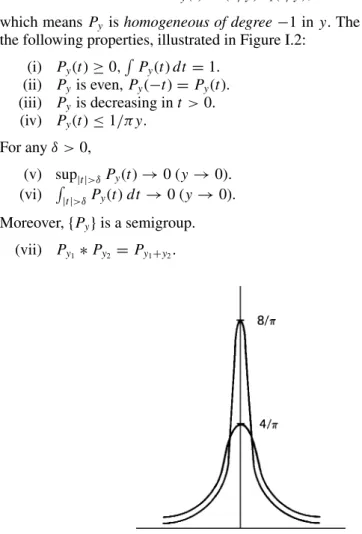
Poisson Integrals

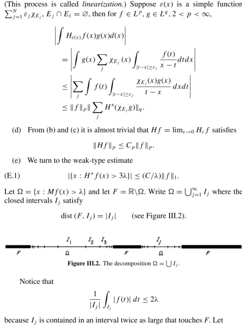
Hardy–Littlewood Maximal Function
Nontangential Maximal Function and Fatou’s Theorem
Subharmonic Functions
Notes
Exercises and Further Results
Definitions
Blaschke Products
Maximal Functions and Boundary Values
The Nevanlinna Class
Inner Functions
Beurling’s Theorem
Preliminaries
The L p Theorems
Conjugate Functions and Maximal Functions
Dual Extremal Problems
The Carleson–Jacobs Theorem
The Helson–Szeg¨o Theorem
Interpolating Functions of Constant Modulus
Parametrization of K
Nevanlinna’s Proof
Maximal Ideal Spaces
Inner Functions