1
Ch. 4. The Various of New Trade Theory Model
1. Skilled and unskilled labor with Core- periphery Model
That make the CP model analytically solvable in the sense that it is possible to derive closed form
solutions for the endogenous variables.
Reference:
Ottaviano, G., and R. Forslid (2003), “An analytically solvable core-periphery model,” Journal of Economic Geography, 3, 229-240.
2
Solvability is achieved by introducing skill
heterogeneity between workers and by coupling a higher level of skill with higher interregional mobility.
This is in line with empirical evidence, which suggests a significantly higher geographical
mobility of skilled compared to unskilled workers (Shields and Shields, Journal of Economic Surveys, 3, 277-304, 1989).
3
The footloose entrepreneur model
The economy consists of two regions, 1 and 2.
There are two factors of production, skilled and unskilled labor.
Each worker supplies one unit of his type of labor inelastically.
4
Total endowments are H and L for skilled and unskilled labor respectively so that H1+H2=H and L1+L2=L, where Hi and Li are the endowments of the two factors in region i.
Skilled workers can be thought of as self-
employed entrepreneurs who move freely between regions, and we will therefore refer to to the model as the ‘footloose entrepreneur’ (FE)model.
5
On the demand side, the consumers’ preferences in country i are defined over two final goods, a
horizontally differentiated good X (manufactures) and a homogenous good A (agriculture).
(4.1)
(4.2)
1 ,
i i
i X A
U
, )
) (
( ( 1)/ /( 1)
d s ds X
N s
i i
6
n1+n2=N
is both the elasticity of demand of any variety and the elasticity of substitution between any two varieties.
1
. 2 , 1
2 ,
L w H i
Y i i
7
The representative consumer in country i maximizes utility (4.1) subject to the following budget constraint:
(4.6)
is the price of the agricultural good.
Turning to the supply side, firms in sector A produce a homogenous good under perfect competition and
constant returns to scale and employ only unskilled labor.
, Y A
p ds
) s ( d ) s ( p ds
) s ( d ) s (
p A i i
n
s s n
ji ji
ii ii
i j
p A
8
Firms in sector X are monopolistically
competitive and employ both skilled and unskilled workers under increasing returns to scale.
Product differentiation ensures a one-to-one relation between firms and varieties.
9
A firm incurs a fixed input requirement of units of skilled labor and a marginal input
requirement of units of unskilled labor.
The total cost of production of a firm producing the output is given by
(4.7)
i L
i i
i
i
( x ) w w x
TC
xi
10
2. Capital and Immobile labor with Core-periphery Model
That make the CP model analytically solvable in the sense that it is possible to derive closed form
solutions for the endogenous variables by using the Capital input.
Reference:
Martin, P. and C.A. Rogers, 1995, “Industrial Location and Public Infrastructure,” Journal
International Economics 39, 335-351
11
Solvability is achieved by introducing capital as production inputs which is free mobile
between countries (regions), while the workers specify as the variable production inputs and which is assumed as immobile between
countries (regions)
12
The footloose capital model
The economy consists of two regions, 1 and 2.
There are two factors of production, capital and unskilled labor.
Each worker supplies one unit of his type of labor inelastically, the labor can work in the
manufacturing sector as variable production inputs or work in the agricultural sector.
13
Utility Function: the same as previous,
On the demand side, the consumers’ preferences in country i are defined over two final goods, a
horizontally differentiated good X (manufactures) and a homogenous good A (agriculture).
(4.1)
(4.2)
1 ,
i i
i X A
U
, )
) (
( ( 1)/ /( 1)
d s ds X
N s
i i
14
A firm incurs a fixed input requirement of
units of capital and a marginal input requirement of units of unskilled labor.
The total cost of production of a firm producing the output is given by
(4.7)
i L
i i
i
x r w x
TC ( )
xi
15
n1 + n2 = N
is both the elasticity of demand of any variety and the elasticity of substitution between any two varieties.
1
. 2 , 1
, )
1
(
r kK r k K w L i
Y
i i j i i
16
3. Input-Output Linkage Model
Specify the relationship among the various
manufacturing industries has the input-output linkage.
Reference:
Krugman, P.R. and J.V. Venables, 1995,
“Globalization and the Inequality of Nations,” Quarterly Journal of Economics 110, 857-880.
17
Assumptions:
1. Two regions: North, South
Two sectors: Manufacture, Agriculture
There are no inherent difference between regions, they are equally proficient in both sectors.
2. The labor is immobile (or far less mobile) between nations, but is free mobile
between two sectors in the same region.
18
3. Each region can produce two kinds of goods:
(1).Agricultural goods:
Produced homogenous good with constant return to scale in perfect competitive market.
(2).Manufactured goods:
Produced differentiated goods subject to increasing return to scale based on the Dixit-Stiglitz
monopolistic competition model.
(2-1).Final goods: sold to consumers
(2-2).Intermediate goods: used as inputs in production of other manufactures
19
4. The production in manufacturing sector use labor and a composite manufacturing
intermediate good to produce output.
5. We make the major simplifying assumption that the composite intermediate good is the same as the composite consumption good.
Thus, the price index of the intermediate
good is the same as the price index of the
composite manufacturing goods.
20
The structure of the model
Final consumption
Import the manufactured goods from the other Regions as intermediated inputs
Intermediated inputs in the same region
Constant
Return to Scale
Monopolistic Competition
Cobb-Douglas Utility Function Labor
input
Labor input
Agricultural Goods
Agricultural Sector Manufactured Sector
Manufactured Goods
Export the manufactured goods to the other region as intermediated inputs
21
Basic stories:
1. Transportation cost between the two nations (regions) are very high.
Each nation (region) will produce both
manufactured and agricultural goods and will be essentially self-sufficient.
2. Transportation cost gradually reduce, there will be the possibility of trade between the nations (regions). If there are many differentiated
manufactured product, then some two-way trade in manufactured goods will arise.
22
M M
M lM
xMinM TC Q x wl
,
s.t. q (xM)l1M
(5.9) Each firm’s objective function is choosing
and to minimize its total production cost, subject to its total output q, that is
] )
1 ( ) / 1 (
[ M
M n X
x
) )
/ 1 (
( M
M n L l
23
Suppose that one nation (region) for some reason has a larger manufacturing sector than the other.
(1). Backward linkages:
This region offers a large market for intermediate
goods, and thus makes the region, other things equal, a more attractive place to locate production of such
goods.
(2). Forward linkages:
If one region produces a greater variety of
intermediate goods than the other, better access to
these goods will, again other things equal, mean lower costs of production of final goods.
24
This is the Marshall’s second reason for spatial agglomeration, the availability of specialized inputs and services, seems straight forward
enough. A localized industry can support more specialized local supplies which in turn makes that industry more efficient and reinforces the localization (Krugman 1991, p49).
3. When transportation cost fall below some critical point then the world economy will spontaneously organize itself into an industrialized core and a deindustrialized periphery.
25
Spatial Agglomeration Economies
Provide the better accessibility for production of final goods Attract more
firms
Produce more
intermediate goods
Attract more firms Demand more
intermediate inputs
Offers a large market for intermediate goods
Backward Linkages
Forward Linkages
26
4. Upstream-Downstream Vertical Linkage Model
This framework specifies the relationship
among the various manufacturing industries has the clarify upstream and downstream vertical linkage.
27 References:
1. Venables A. J., 1995,“Economic Intergration and the location of firms,” American Economic Review 85, 296-300.
2. Venables A. J., 1996, “Equilibrium Locations of Vertically Linked Industries,” International Economic Review 37, 341-359.
3. Krugman, P., and Venables A. J., 1996, “Intergration, Specialization, and adjustment,” European Economic Review 40, 959-967.
28
Introduction
The choice of firm’s location determined by:
1. Production cost,
2. The accessibility to market (i.e. trade
cost)
29
(i) Low trade cost
Firms are highly sensitive to production cost difference and industries are “footloose”.
(ii) High trade cost
Firms are tied to markets and their location
decisions are much less sensitive to production costs.
(iii) Intermediate trade cost
The distribution of firms in an imperfectly
competitive industry is skewed towards locations with ease market access. (Krugman, 1980, AER)
30
(1) Forward Linkages:
Firms cluster together,
Produce more intermediate goods,
Provided the better accessibility for production of final goods,
Attract more firms to locate in the same region.
31
(2) Backward Linkage:
More firms locate in the same region,
Demand more intermediate inputs,
Offers a large market for intermediate goods,
Attract more firms to agglomerate together.
32
The concerned problem of locations choice for vertically linked industries
If industries are vertically linked through an input- output structure, then where do the upstream and downstream industries locate?
33
The determination of equilibrium location for vertically linked industries.
The balance between the centripetal force
and the centrifugal force.
34
1. Centripetal force (i.e., Agglomeration force)
Demand linkage + Cost linkage
(1) Demand linkage (for the firms in the upstream industry)
Market access considerations draw the
upstream industry to the locations where there are relatively many downstream firms.
(2) Cost linkage (for the firms in the downstream industry)
Firms in the downstream industry will have lower costs if they locate where there relatively
many upstream firms, since they can save trade cost on their intermediate inputs.
35
2. Centrifugal forces
(1) Immobile production factors,
(2) The location of final consumer demand.
36
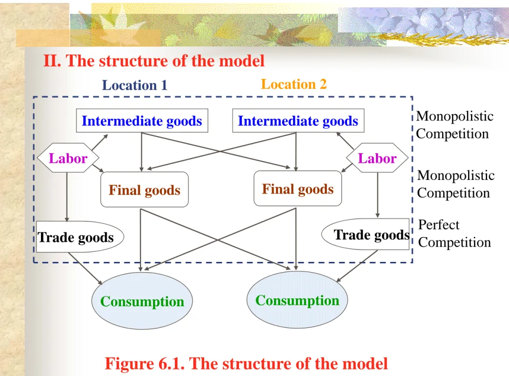
Assumptions and the structure of the model
I. Assumptions
Each economy has three industry sectors and a consumption sector:
(i) One is perfectly competitive, producing a
tradeable good to provide final consumption, which we use as numeraire.
(ii) The upstream industry employ labors to produce an intermediate good by monopolistic
competition to provide the final good as production inputs.
37
(iii) The downstream industry use labor and intermediate good as input to produce final good to provide consumers as final
consumption, also in the downstream
industry, firms behave a standard model of monopolistic competition with product
differentiation.
38
(iv) Households in each economy consume tradeable good and final good (downstream industry) by
Cobb-Douglas utility function.
(v) The labors in each economy are identical, and which can be employed in producing tradeable goods, intermediate goods, or final goods.
39 II. The structure of the model
Figure 6.1. The structure of the model
Intermediate goods Intermediate goods
Final goods
Trade goods
Final goods
Location 1 Location 2
Consumption Consumption
Monopolistic Competition
Perfect
Competition Monopolistic Competition
Labor Labor
Trade goods
40
Demand Side of Manufacturing Goods in k Industry
I. Demand Side of k Goods:
(6.1) where
total demand for goods k which is formed by CES over N varieties,
the demand for each variety,
the elasticity of demand for a single variety for industry (or good ) k.
1 1
1
]
[
k
k k
N k
i
i k
i x
X
k : Xi
i : x
k:
41
If industry k may contain firms at two locations i and j with number and , then equation (6.1) can be rewritten by:
(6.2)
where is the quantity of a particular variety of
industry k output produced in j and sold in i.
k
ni nkj
1 1
1
k
k k
k k
k
] )
x ( n )
x ( n [
Xik ik iik kj kji
: xkji
42
II. Supply Side of Manufacturing Goods in k Industry
Production function:
(6.22) Where
denote the total inputs for produce q quantity of goods k in location i,
denote the fixed input.
the quantity of each variety should be produced for industry k at location i, , and this condition implies that the total supply equals the total demand for firm locates in location i.
k i k
k
i f q
y
k : yi
k : f
k : qi
] x ) t ( x
q
[ ik iik k ijk
43
5. The Framework with Quadratic Utility function An alternative model of agglomeration is developed to examine the trade between countries and display the main features of the recent economic geography, and which is analytically solvable by means of simple
algebra.
Specify the utility function by Log-linear function form to substitute the conventional CES function form
.
44
Main Reference:
Ottaviano, G., and T. Tabuchi, and J.-F.
Thisse (2002), “Agglomeration and trade
revisited,” International Economic Review,
43, 409-435.
45
The other references:
Picard., P. M. and D. Z. Zeng (2005),
“Agricultural sector and industrial
agglomeration,” Journal of Development Economics, 77, 75-106.
Tabuchi. T. and J.-F. Thisse (2006),
“Regional specialization, urban hierarchy, and commuting costs,” International
Economic Review, 47(4), 1295-1317.
46
First, the main tool used in the new economic geography is a particular version of the
Chamberlinian model of monoplolsitic competition developed by Dixit and Stiglitz (1977, AER) in which consumers love variety and firms have fixed
requirements for limited productive resource.
(1). Love of variety is captured by a CES utility function that is symmetric in a bundle of
differentiated products.
(2). Each firm is assumed to be a negligible actor in that it has no impact on overall market conditions.
47
Second, the transportation cost is specified by “iceberg form”, that is, transportation is
modeled as a costly actively that uses the
transported good itself. Namely, a certain
fraction of the good melts on the way.
48
The combination of both assumptions yields that a demand system has a own-price elasticity of demand with constant, and identical to the
elasticity of substitutions, and equal to each other across all differentiated products.
This entails equilibrium prices that are
independent of the spatial distribution of firms
and consumers
49
5.1 The limitation of the conventional model:
1. Though this setting is convenient from an analytical point of view, such a result conflicts with research in spatial pricing theory.
2. The demand elasticity varies with distance while prices change with the level of demand elasticity and the intensity of competition.
3. The assumption of the iceberg trade cost is
unrealistic.
50
5.2 The Motivation of this Model:
1. To develop a complementary modeling strategy to overcome the previous limitation,
2. The alternative framework still present a
model of agglomeration and trade, and display
the main features of core-periphery as shown in
the literature.
51
5.3 The setting of this framework:
1. Consumers’ preferences are not CES as shown in the conventional literature, the quadratic utility function is adopted to specify the preferences for variety.
2. The firms are still considered as negligible actors, and employ a broader concept of
equilibrium than the one in Dixit and Stiglitz.
3. The trade cost are assumed to absorb
resources that are different from transported good.
52
Taking together of previous modifications:
1. This specifications allow us to disentangle the economic meanings of the various parameters, thus leading to clear-cut comparative static results that are likely to be easier to test than those based on Dixit and Stiglitz (1977).
2. It also entails elasticities of demand and substitution that vary with prices, while
equilibrium prices now depend on all the
fundamentals of the market.
53
5.4 The advantage of this model:
1. It can analytically solve the interesting results obtain by Krugman (1991).
2. It also allows us to study forward-looking location decisions and to determine the exact domain in which expectations matter for
agglomeration.
3. It is sufficiently flexible to establish a bridge
between the new economic geography and urban
economics.
54
5.5 The assumptions and the structure of the model:
1. Assumptions:
(1). The economic space is made of two countries (or regions), called H and F.
(2). There are two production factors, called A and L.
Factor A (farmers) is evenly distributed across countries and spatially immobile. Factor L (workers) is mobile
between the two countries, and denotes the shares of this factor located in the country H.
] 1 , 0
[
55
(3). There are two goods in the economy. The first good is homogenous. Consumers have a positive initial
endowment of this good that is also produced using factor A as the only input under constant return to scale and
perfect competition. And this good can be traded freely between countries and is chosen as the numéraire.
(4). The other good is horizontally differentiated product;
it is produced by using factor L only, and under increasing returns to scale and imperfection competition.
56
(5). There is a continuum N of potential firms, so that all the unknowns are described by density functions.
(6). There are no scope economies so that, due to
increasing returns to scale, there is one-to-one relationship between firms and varieties. Since each firm sells a
differentiated variety, it faces a down-ward-sloping demand.
(7). Each variety can be traded at a positive cost of units of the numéraire for each unit transported from one country to the other, regardless of the variety, where accounts for all the impediments to trade.
57
Utility function:
Preferences are identical across individuals and described by a quasi-linear utility with a quadratic subutility
q(i): denotes the consumption quantity of variety : is the quantity of the numeraire,
: expresses the intensity of preferences for the different product,
, )
2 ( )]
( 2 [
) ( ])
, 0 [ ), (
;
( 0
2 0
0
2
0 q i i N 0 qi di qi di q i di q
q
U N N N
(7.1)], , 0 [ N i
q0
58
: implies that consumers are biased toward a
dispersed consumption of varieties, i.e., this quadratic utility function exhibits consumers love of variety as long as .
For a given value of , the parameter expresses the substitutability between varies, the higher implies the closer substitutes the varieties. When ,
substitutability is perfect. Indeed, equation (7.1)
degenerates into a utility function that is quadratic in total consumption , which is exactly what one would expect with a homogeneous product.
di i
N q
0 ( )59
Any individual is endowed with one unit of labor (of type A or L), and units of the numeraire. His budget constrain then can be written as follows:
(7.2) where y is the individual’s labor’s income, p(i) is the price of variety, and the price of the agriculture
good is normalized to one. The initial endowment is to be sufficiently large for the equilibrium consumption of the numeraire to be positive for each dividual.
0 0
0N p(i)q(i)di q y q
0 0 q
q0
60
Maximization the consumer’s utility (7.1) subject to the budget constrain (7.2), and solving the first-order condition with respect to q(i) yields:
(7.3) Similarly, we have
(7.4) Substituting (7.4) into (7.3) to yield the demand for variety as
(7.4)
( ) ( ) ( ) 0 ( )
0 q j dj q p i
i
q N
N)
(0, i
dj i
q j
q c
i bp a
i
q( ) ( ) N [ ( ) ( )]
0
) ( )
( )
( )
( 0
0 q i di q p j
j
q N
61
1 { ( ) ( )}
)
(i 0 q j dj p i
q N
)}
( )]
( )
( 1 [
1 {
0
0N N q i di p j dj p i
)}
( )]
( )
( [
1 {
0
0 q i di p j p i
N
N N N
) ) (
( ] 1 ) ) (
) ( ) (
( )
(
] ) 1 (
[
2 0 2
2 2
2 N q i p j dj p i
N N
) ( ) (
) ( )
( ]
) 1 (
[ )
( )
( 0
2 2
2q i N N q i N p j dj p i
62
) ( )]
( )
( [
) ( ) (
] ) 1 (
[ )
( ] )
[(
0 2
2 2
i p N dj
i p j
p
i p N
i q N
N
) ( )]
( )
( [ )
( ) (
] ) 1 (
[
) ( ] )
][(
) [(
0 p j p i dj N p i
i p N
i q N N
N
dj i p j
p i
p N
N
i q N N
N [ ( ) ( )]
) ( ] ) 1 (
[ ] ) 1 (
[
) ( ] )
][(
) [(
0
dj i p j
N p N
i N p
i N q
N [ ( ) ( )]
] ) 1 (
][(
) 1 (
[(
) ) (
1 (
1 )
1 ) (
(
0
63
Thus, we have the demand for variety as follows:
(7.5) Where,
N)
(0, i
dj i
q j
q c
i bp a
i
q( ) ( ) N [ ( ) ( )]
0
) 1
(
a N
( 1) 1
b N
] ) 1 (
][(
) 1 (
[(
N c N
64