The fact that the order of the data does not matter for econometric analysis is a central feature of cross-sectional data sets obtained by random sampling. We will use the methods and insights from the cross-sectional analysis in the rest of the text.
CAUSALITY AND THE NOTION OF CETERIS PARIBUS IN ECONOMETRIC ANALYSIS
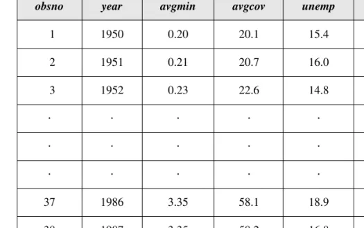
If we can control for enough other factors related to employment, then we can still hope to estimate the ceteris paribus effect of the minimum wage on employment. Other issues, such as trends and seasonality, arise in the analysis of time-series data but not cross-sectional data.
DEFINITION OF THE SIMPLE REGRESSION MODEL Much of applied econometric analysis begins with the following premise: y and x are
When related to (2.1), the variables y and x have several different names used interchangeably, as follows. y is called the dependent variable, explanatory variable, response variable, predictor variable, or regressor. The agricultural researcher is interested in the effect of fertilizer on yield, holding other factors fixed.
DERIVING THE ORDINARY LEAST SQUARES ESTIMATES
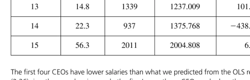
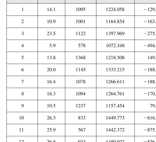
These are not the same as the errors in (2.9), a point we return to in Section 2.5.) The fitted values and residuals are given in Figure 2.4. For the population of CEOs, let y be the annual salary (salary) in thousands of dollars.
MECHANICS OF OLS
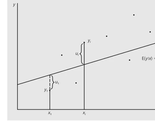
In other words, no data point may actually lie on the OLS line. Sometimes the explanatory variable explains a significant part of the sample variation of the dependent variable.
UNITS OF MEASUREMENT AND FUNCTIONAL FORM
This implies that a 1 percent increase in firm sales increases CEO pay by about 0.257 percent—the usual interpretation of an elasticity. It is also useful to note what happens to the intercept and slope estimates if we change the units of measurement of the dependent variable when it appears in logarithmic form.
EXPECTED VALUES AND VARIANCES OF THE OLS ESTIMATORS
PROOF: In this proof, the expected values are conditional on the sample values of the independent variable. It turns out that the variance of the OLS estimators can be calculated under Assumptions SLR.1 to SLR.4.
REGRESSION THROUGH THE ORIGIN
Do you think that simple regression provides an unbiased estimator of the ceteris paribus elasticity of price with respect to dist. Likewise, the method of ordinary least squares is widely used for estimating multiple regression model parameters.
MOTIVATION FOR MULTIPLE REGRESSION The Model with Two Independent Variables
Thus, multiple regression analysis can be used to build better models for predicting the dependent variable. In Section 3.2, we demonstrate how to estimate the parameters in the multiple regression model using the method of ordinary least squares.
MECHANICS AND INTERPRETATION OF ORDINARY LEAST SQUARES
The independent variables here have two subscripts, i followed by 1 or 2. The i subscript refers to the observation number. We call ˆ0 the OLS intercept estimate and ˆ1, …,ˆk the OLS slope estimates (corresponding to the independent variables x1, x2, …, xk). This means that the sample mean, y¯,. explains more the variation in the yi than the explanatory variables.
THE EXPECTED VALUE OF THE OLS ESTIMATORS We now turn to the statistical properties of OLS for estimating the parameters in an
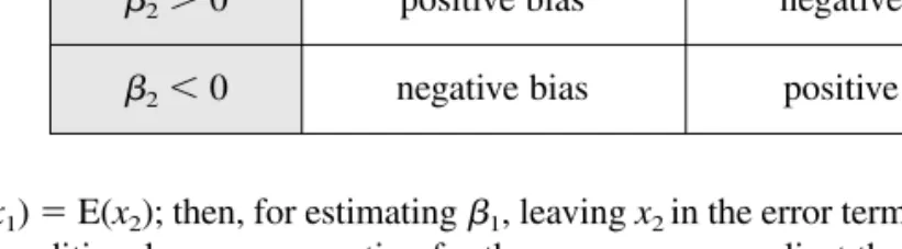
A serious drawback of regression through the origin is that if the intercept 0. in the population model is different from zero, the OLS estimators of the slope parameters will be biased. As in the simple regression case, the expectations depend on the values of the independent variables in the sample, but we do not show this conditioning explicitly. Even in the fairly simple model above, it is difficult to determine the direction of the bias.
THE VARIANCE OF THE OLS ESTIMATORS
Assumption MLR.5 means that the variance in the error term, u, conditional on the explanatory variables, is the same for all combinations of outcomes of the explanatory variables. 2 is the proportion of the total variation in xj that can be explained by the other independent variables in the equation. 2 .9 means that 90 percent of the sample variation in xj can be explained by the other independent variables in the regression model.
EFFICIENCY OF OLS: THE GAUSS-MARKOV THEOREM
We already know that the failure of the zero conditional mean assumption (MLR.3 Assumption) causes OLS to be biased, so Theorem 3.4 also fails. R2 is the portion of the sample variation in the dependent variable that is explained by the independent variables, and serves as a measure of goodness-of-fit. Why do we need to leave one of the tax share variables out of the equation? ii) Carefully interpret 1.
Now, under assumptions MLR.2 and MLR.4, the expected value of each ui, given all independent variables in the sample, is zero.
1 冹 2
1 冹
SAMPLING DISTRIBUTIONS OF THE OLS ESTIMATORS
In section 3.4 we obtained the variances of the OLS estimators under the Gauss-Markov assumptions. Knowing the expected value and variance of the OLS estimators is useful for describing the precision of the OLS estimators. When we determine the values of the independent variables in our sample, it is clear that the sampling distributions of the OLS estimators depend on the underlying distribution of the errors.
TESTING HYPOTHESES ABOUT A SINGLE POPULATION PARAMETER: THE t TEST
The statistic we use to test (4.4) (against any alternative) is called "the" t-statistic or "the" t-ratio of ˆ. 4.5) We put “the” in quotation marks because, as we will see shortly, a more general form of the t-statistic is needed to test other hypotheses about j. Our first instinct might be to construct "the" t-statistic by taking the coefficient on log(entry) and dividing it by its standard error, which is the t-statistic reported by a regression package. Thus, if hremp increases by 5—each employee is trained 5 more hours per year—the scrap rate is estimated to decrease by 5(2.8) 14%.
CONFIDENCE INTERVALS
A model that explains the price of a good in relation to the good's characteristics is called a hedonic price model. However, it is important to remember the ceteris paribus nature of this coefficient: it measures the effect of another bedroom, the size of the house and the number of bathrooms fixed. If heteroscedasticity is present—for example, in the previous example, if the variance of log(price) depends on one of the explanatory variables—then the standard error is not valid as an estimate of sd(ˆ . j) (as we discussed) in Section 3.4), and the confidence interval calculated using these standard errors will not really be a 95% CI.
TESTING HYPOTHESES ABOUT A SINGLE LINEAR COMBINATION OF THE PARAMETERS
Considering the size and number of bedrooms, another bathroom is expected to increase the house price by around 15.8%. Remember that we must multiply the coefficient on bthrms by 100 to turn the effect into a percent.) The 95% confidence interval for bthrms is. Unfortunately, the regression results in equation (4.21) do not contain enough information to obtain the standard error of ˆ. The coefficient on the new variable, totcoll, is the same as the coefficient on univ in (4.21), and the standard error is also the same.
TESTING MULTIPLE LINEAR RESTRICTIONS
Write the unconstrained model with k independent variables as the number of parameters in the unconstrained model is k1. Suppose we have q exclusion restrictions to test: that is, the null hypothesis states that q of the variables in (4.34) have zero coefficients. In most applications, it seems more convenient to use a form of the F-statistic that can be calculated using the R-squares of the restricted and unrestricted models.
REPORTING REGRESSION RESULTS
General multiple linear restrictions can be tested using the residual sum-of-squares form of the F statistic. In terms of model parameters, state the null hypothesis that after controlling for sales and profits, ros has no effect on CEO pay. 2 denote the OLS of estimators 1 and 2. 2) in terms of variances ˆ. 2 and the covariance between them.
CONSISTENCY
Similarly, the fact that OLS is the best linear unbiased estimator under the full set of Gauss-Markov assumptions (MLR.1 to MLR.5) is a finite sample property. In Chapter 4, we added the classical linear model Assumption MLR.6, which states that the error term u is normally distributed and independent of the explanatory variables. One practically important finding is that even without the normality assumption (Assumption MLR.6), t and F statistics approximate t and F distributions, at least in large sample sizes.
ASYMPTOTIC NORMALITY AND LARGE SAMPLE INFERENCE
The exact normality of the OLS estimators critically depends on the normality of the distribution of the error, u, in the population. The df in the unrestricted model does not play a role due to the asymptotic nature of the LM statistic. But you should be aware of the LM metric as it is used in applied work.
ASYMPTOTIC EFFICIENCY OF OLS
We have shown in the simple regression case that, under the Gauss-Markov assumptions, the OLS estimator has a smaller asymptotic variance than any estimator of the form (5.17). We also showed that the LM statistic can be used instead of the F statistic for exclusion constraint testing. We outline a proof of the asymptotic normality of OLS (Theorem 5.2[i]) in the simple regression case.
EFFECTS OF DATA SCALING ON OLS STATISTICS In Chapter 2 on bivariate regression, we briefly discussed the effects of changing the
This chapter brings together several issues in multiple regression analysis that we could not easily address in previous chapters. These topics are not as fundamental as the material in Chapters 3 and 4, but they are important for applying multiple regression to a wide variety of empirical problems.
MORE ON FUNCTIONAL FORM
Applying simple algebraic properties to the exponential and logarithmic functions gives the exact percentage change in the predicted y as. Using the log means we are looking at the percentage change in the unemployment rate: log(9) log(8) ⬇ .118 or 11.8%, which is the logarithmic approximation of the actual increase of 12.5%. If this point is beyond all but a small percentage of people in the sample, then this is not a major concern.
MORE ON GOODNESS-OF-FIT AND SELECTION OF REGRESSORS
Because of the notation used to denote the adjusted R-squared, it is sometimes called R-bar squared. This test does not allow us to decide which of the variables has an effect. Equation (6.26) shows that log(sales) and spawn explain about 28.2% of the variation in log(salary).
PREDICTION AND RESIDUAL ANALYSIS
However, there is one case that is obvious: We should always include independent variables that affect y and are uncorrelated with all the independent variables of interest. If these factors affect demand and are uncorrelated with price, the standard error of the price variable will be smaller, at least in large samples. However, it is worth bearing in mind that when these variables are available, they can be included in a model to reduce the error variance without inducing multicollinearity.