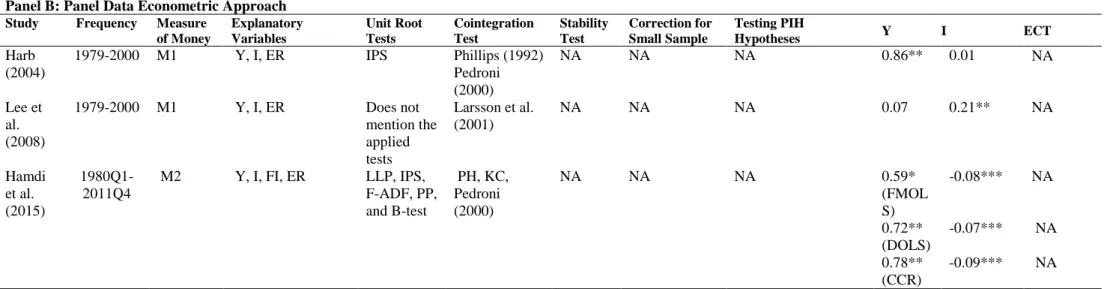
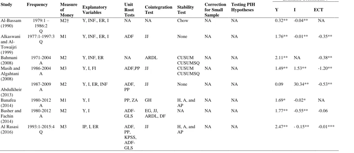
The researcher followed the partial adjustment model to estimate the money demand function for Saudi Arabia. Masih and Algahtani (2008) considered the long-run structural modeling technique (LRSM) initiated by Pesaran and Shin (2002) to estimate and assess the stability of the long-run money demand function in Saudi Arabia. Nevertheless, the estimated money demand function with real private consumption is in line with theoretical expectations.
Similarly, the estimated coefficient for the money demand function for the individual countries is in line with the theoretical expectation.
Theoretical Framework
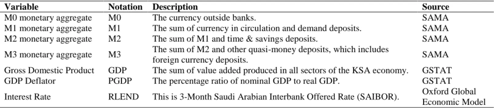
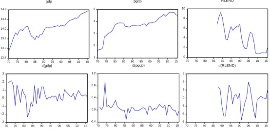
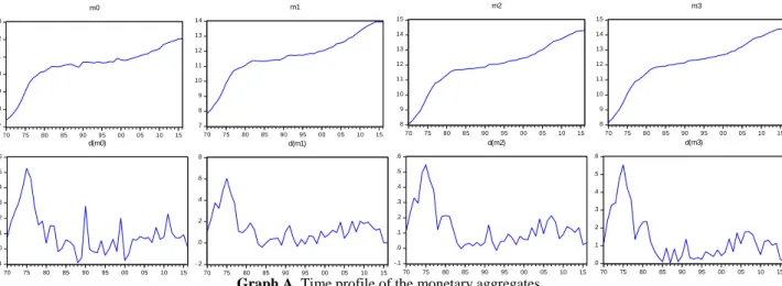
Data
Econometric Methods
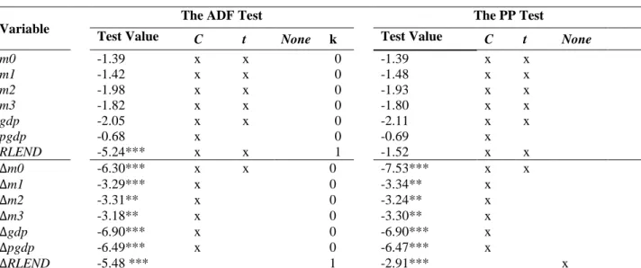
Unit Root Test
Therefore, it is important to first check its stationarity through UR testing to avoid false results. The most commonly used UR tests are the Augmented Dickey Fuller (ADF) test (Dickey and Fuller, 1979) and the Philips-Perron (PP) test (Phillips and Perron, 1988), although many UR tests are available. One fails to reject the null hypothesis of UR if this value is less than the critical ADF values, in absolute terms, at different levels of significance, and it means that 𝑦𝑡 has UR and is therefore not stationary.
If this value is greater than the critical ADF values, in absolute terms, at different levels of significance, then the null hypothesis can be rejected and it means that 𝑦𝑡 is not non-stationary. The only difference between the PP test and the ADF test is that to remove the serial correlation problem in the residuals, the former uses non-parametric statistical methods, but does not use dependent variable delays. The Johansen Cointegration Method The classical cointegration theory states that if variables are non-stationary and their order of integration is the same.
The Johansen Cointegration MethodThe classic cointegration theory articulates that if variables are non-stationary and their integration order is the same,
Once the Johansen test suggests only one cointegration relationship between the variables, other cointegration tests such as the EG and the ARDLBT can be used or their long- and short-term estimates can be performed as a robustness test. The former indicates the importance of the cointegration relations in the individual equations of the system and of the speed of adjustment to disequilibrium, while the latter represents the long-term equilibrium relation, so that Π = αβ′. Johansen's reduced rank regression approach to testing for cointegration first estimates the matrix Π in an unrestricted form and then tests whether the restriction implied by the reduced rank of Π can be rejected.
In particular, the number of independent cointegrating vectors depends on the rank of Π, which in turn is determined by the number of its characteristic roots that are different from zero. Note that tests of significance, stationarity and weak exogeneity are usually performed in the Johansen framework, using the estimated VECM (Johansen, 1992a, b). If a given variable in the long run is significant, then the null hypothesis of the corresponding β is zero can be rejected.
If a given variable is weakly exogenous, this implies that the null hypothesis of corresponding α is zero cannot be rejected. Johansen (2002) discussed that in the case of small samples, the Max Eigenvalue or Spoor test statistics are biased to reject the null hypothesis of no cointegration. 𝑇 correction to the maximum eigenvalue or trace test statistics; where k is the lag length of the underlying Vector Autoregressive (VAR) model in levels and n and T are the number of endogenous variables and observations, respectively.
Error Correction Model with the General to Specific Modeling Strategy This sub-section briefly describes that if the variables are cointegrated, then how short-
Error correction model with the general modeling strategy in the specification This sub-section briefly describes that if the variables are cointegrated, then how short-. The maximum delay order in the general ECM can be specified using different approaches, such as a time-dependent rule, information criteria (such as Schwarz and Akaike), statistical significance of the maximum delay order, and series frequency times used (see Perron, 1989; Newey and West, 1994; Ng and Perron, 1995). For example, Perron (1989) suggested that if the frequency is quarterly and the number of observations is small, then the maximum lag order of four should be chosen.
Note that if x is weakly exogenous to the cointegrating system, then estimating equation (6), where we have the contemporaneous value of x, with OLS is possible without loss of useful information (see De Brouwer and Ericsson, among others). One approach, but it may be with a loss of useful information, is to exclude the contemporaneous value of x from the ECM and estimate it with OLS. Another approach that does not result in the loss of any useful information is to estimate a simultaneous system of ECM equations for y and x, where we have simultaneous values of both variables.
However, another approach is that we still have the simultaneous value of x and thus no loss of useful information, but the final single ECM equation of y must be estimated by two-stage OLS (TSLS) to address an issue of possibly endogenous. Note that it is important to first check whether the simultaneous value of x in the final ECM specification causes an endogeneity problem. If the test shows that the contemporaneous value of x is not endogenous, then there is no benefit from TSLS estimation and it is proved econometrically that OLS is the best estimator.
Empirical Analysis
Cointegration Tests Results
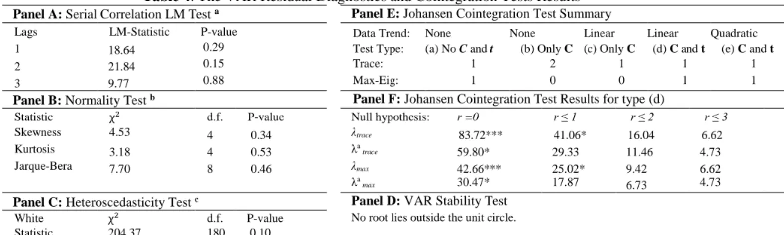
However, the long-run and short-run analyzes show that aggregate M2 is a more appropriate measure of the Saudi Arabian economy in the given time period. Furthermore, the trend is statistically significant in the long-run equation as reported in Panel B of Table 5. The long-run money demand equation corresponding to version (d) is presented in Panel A of Table 5.
Panel H: Long-run equation in the case of price and income homogeneity and weak price exogeneity. The theory of money demand articulates that money demanded and price may be in a one-to-one relationship in the long run. In the case of price homogeneity hypothesis, the coefficients on RLEND and TREND have the same values as they have in the unrestricted long-run equation, while for gdp it is very similar to each other.
Then we tested another hypothesis derived from the theory of money demand, which states that it may be possible for money demanded and income to be in a one-to-one relationship in the long run. We would prefer this specification of the long-run equation where we have a homogeneity hypothesis for price and income incorporated. Finally, we reached the long-run money demand specification where we have price and income homogeneity and weak exogeneity of the price.
Short-run Analysis
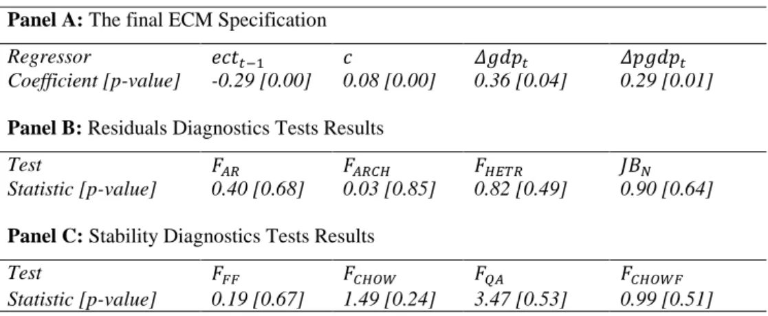
It appears that only price is slightly exogenous to the system at the 10 percent significance level as shown in panel G of the table. Although it is at the 10 percent significance level, due to the explanations given above, we would accept it as a research decision. The final ECM specification of 𝛥m2 estimated using OLS is reported in Panel A of Table 6.
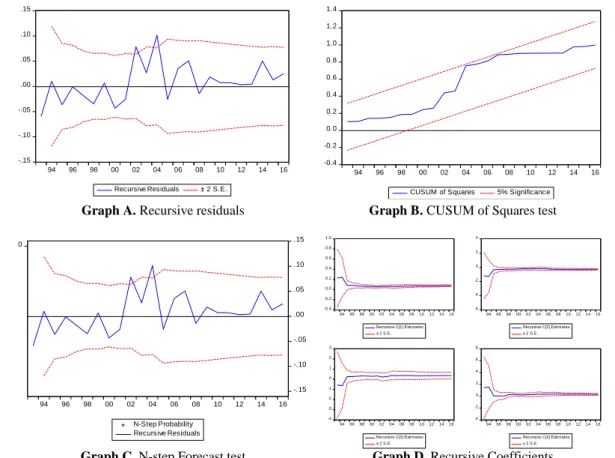
Note that in terms of the final robustness check of the ECM specification, we estimated the overall ECM using the Stepwise Regression method. It shows that the residuals of the final ECM specification do not have any problem with serial correlation, ARCH effect and heteroscedasticity, and are also normally distributed. Finally, we performed several tests to verify the stability of the final ECM specification of the money demand.
The last graph illustrates that all four estimated coefficients of the final ECM specification are very stable over time. The obtained sample value of the Average Wald F statistic of 3.47 with the rather high p-value indicates that there is no break in the money demand relationship. The remaining five metrics of the Quandt-Andrews test, such as the Average and Maximum Likelihood Ratio F stats and Maximum Wald F stats, also show no break in the relationship.
Discussion of the Empirical Results
Thus, we conclude that the jump in 2004 does not cause any structural change neither in the estimated parameters nor in the relationship between the demand for money and its factors. In this regard, the estimated unrestricted long-run money demand equation reported in Panel A of Table 6 shows that, ceteris paribus, a 1 percent increase in GDP, PGDP, and RLEND leads to 0.51 percent, 1.05 percent, and 3 percent increase demand for the monetary aggregate M2 in the long run. The equation also shows that time-varying factors not included in the equation led to a 4% increase in the demand for M2 each year over the period 1989-2016.
After testing the theoretical predictions, we conclude that in the long run, M2 may be in a one-to-one relationship with PGDP and GDP in panel F. Moreover, the empirical analysis shows that this transaction motive has a one-to-one relationship has with M2 in the long run. The positive effect of the price level on the demand for money can be explained in such a way that when the price level is higher in the Saudi economy, goods and services will be more expensive to buy than before.
Whether the interest rate has a negative (or positive) effect on money demand depends on both the interest rate and money demand being considered. All this shows that the long-term relationship between M2 and its determinants is stable and any shocks to this relationship will be temporary in the Saudi economy. It is worth noting that short-term effects of income and price occur less than in the long-term.
Conclusion
Finally, we run a series of different stability tests, as a robustness check, to see if there is a break in the money demand relationship in Saudi Arabia. Finally, we applied several structural break tests to our final ECM because it is important to know whether a given money demand relationship is stable over time. Finally, it is essential for policymakers to understand how the demand for money in Saudi Arabia behaves in both the short and long term.
In particular, maintaining a stable money demand function is a key requirement for predicting the nominal exchange rate based on the monetary exchange rate model. Money demand and supply in Saudi Arabia: An empirical analysis (PhD thesis, University of Leicester). Asymmetric responses of money demand to oil price shocks in Saudi Arabia: A nonlinear ARDL approach.
Essays on structural breaks and stability of the money demand function (PhD dissertation, Kansas State University). Empirical evidence on the long-run money demand function in the Gulf Cooperation Council countries. Estimating Long-Run Demand for Money: An Application of Long-Run Structural Modeling to Saudi Arabia.