Sumit Agarwalis is a financial economist in the research department of the Federal Reserve Bank of Chicago. Christoph Kessleris CEO and works in the Risk Management team at UBS Global Asset Management.
1 Determinants of small business default ∗
Abstract
- Introduction
- Data, methodology and summary statistics
- Data
- Methodology
- Summary statistics
- Empirical results of small business default
- Default behaviours of loans versus lines
- Default behaviours of small versus large credits
- Conclusion
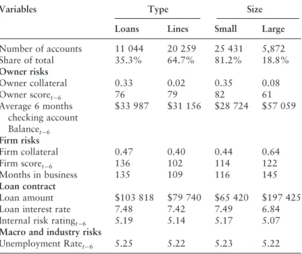
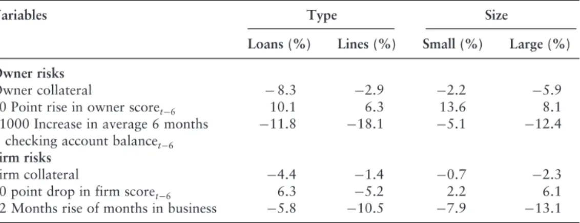
A similar 10-point improvement in corporate credit scores lowers default risk by 6.3% for small business loans, but only 5.2% for small businesses. Similarly, strong collateral lowers the risk of default by 4.4% for loans, but only by 1.4% for lines of credit.
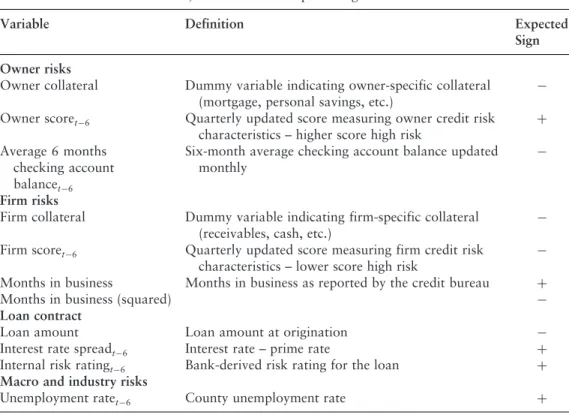
The marginal impact of owner collateral, improving credit risk for the owner and strengthening the owner-bank relationship in reducing the risk of default is significantly greater for loans than for lines of credit. For example, the marginal impact of deteriorating owner credit risk on default probability is greater for small firms, while the marginal impact of deteriorating corporate credit risk on default probability is greater for large firms.
Notes
When distinguishing between small and large business accounts, our results suggest that the economic impact of owner and firm characteristics on small business defaults also differs significantly. Next, we can choose to control them at that time since the start of the sample or delay them 12 months from the default time.
2 Validation of stress testing models
- Why stress test?
- Stress testing basics
- Tradable instruments
- Commercial lending models
- Retail lending models
- Underlying similarities
- Overview of validation approaches
- Subsampling tests
- Random sampling
- Old versus new accounts
- Ideal scenario validation
- Scenario validation
- Cross-segment validation
- Back-casting
- Conclusions
We expect the dependence of the model f on the macroeconomic factors Xt to be the same for all subsets. When the test is performed, the prediction error is an indication of the model accuracy.

3 The validity of credit risk model validation methods ∗
- Measures of discriminatory power
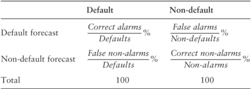
- The contingency table
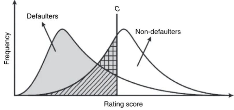
- The ROC curve and the AUROC statistic
- The CAP curve and the AR statistic
- Uncertainty in credit risk model validation
- Confidence intervals for AUROC
- The Kupiers Score and the Granger–Pesaran Test
- Confidence interval for ROC
- Analysis under normality
- Examples under normality
- The construction of ROC confidence intervals
- Analysis under non-normality
- Examples under non-normality
- Bootstrapping
- Optimal rating combinations
- Concluding remarks
The ROC curve is therefore defined as the plot of the off-diagonal element combinations of a contingency table for all possible cut-off points. The CAP curve is constructed from combinations of the CAR (vertical axis) and the total number of defaults and non-defaults (horizontal axis) for all possible cut-offs.
4 A moments-based procedure for evaluating risk forecasting models
- Preliminary analysis
- The likelihood ratio test
- A moments test of model adequacy
- An illustration
- Conclusions
- Acknowledgements
The power of LR hardly improves, asn becomes larger, but the power of moment test improves noticeably. This is as you would expect because the inadequacy of the model is in one of the higher moments that the LR test does not address.
Appendix
- Error distribution
- Two-piece normal distribution
- t-Distribution
- Skew-t distribution
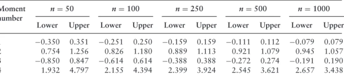
In practice, we would start with the overall significance level and then obtain the associated value using the relationship = 1−1−1/4. For example, if we wanted to include the fifth moment prediction and have an overall significance level, we would choose = 1−1−1/5. We would then add a fifth-moment test comparable to the individual four-moment tests considered in the text and calibrate accordingly.
Once we have the five sets of bound estimates, one for each moment, we will apply the actual test.
5 Measuring concentration risk in credit portfolios
- Concentration risk and validation
- Concentration risk and the IRB model
- Measuring name concentration
- Measuring sectoral concentration
- Numerical example
- Future challenges of concentration risk measurement
- Summary
In summary, the two assumptions of the IRB model necessary for portfolio invariance are closely related to the two types of risk concentration in the portfolio. Furthermore, the IRB model's maturity adjustments can be easily accommodated by including them in the inputs. Concentration risk in credit portfolios is woven into the portfolio's credit risk and is therefore implicitly taken into account in best-practice multi-factor portfolio models used in the industry.
For more details on UL capital in the context of the one-factor model, see Appendix A.1.

Appendix A.1: IRB risk weight functions and concentration risk
See Appendix A.2 for further details on the definition of DF(.), its two components CDI and and the DF surface parameterization. This structural similarity is misleading in that the calibration of the maturity adjustments, which are omitted here, was actually performed in a mark-to-market framework. The UL capital chargeKN ∗ for the total portfolio in the IRB model captures the unexpected loss and is defined by.
For simplicity, maturity adjustments, the dependence of PD on several asset classes, and the requirement to distinguish between an (expected) LGD and an economic decline LGD are omitted in equation 5.10.
Appendix A.2: Factor surface for the diversification factor
The parameter, commonly referred to as asset correlation, is the correlation between the solvency processes of each pair of borrowers. In Garcia Cespedes et al. (2006), the sector factor correlation matrix has only nine parameters instead of S·S−1/2 in the general multifactor model. Therefore, the correlation matrix is fully specified by the weights S of the single common factor.
In the numerical example, the correlation parameters in equation 5.12 are instead taken from the more general matrix.
Appendix A.3
The reason is that they define each sector factor as a weighted sum of a risk factor common to all sectors and a sector-specific risk factor.
6 A Simple method for regulators to cross-check operational risk loss
- Background
- Cross-checking procedure
- Justification of our approach
- Justification for a lower bound using the lognormal distribution
- Conclusion
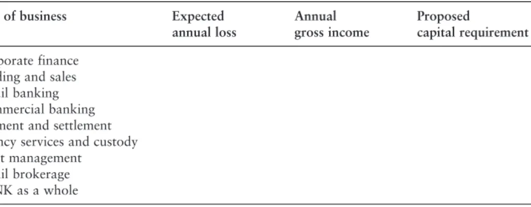
The regulator uses the 99.9th percentile of this distribution to obtain a lower limit for the capital requirement for all values for each of the business lines and for the bank as a whole. For the lognormal distribution, if and are the mean and standard deviation of the underlying normal distribution, then Lower bound function: For each line of business and for the total, the regulator sets L to be a lower bound on the minimum capital requirement based on the 99.9th percentile of the lognormal distribution minus the expected value, respectively, as functions ranging from 0 with 1.
Therefore, the 99.9th percentile of the lognormal value for the same mean and standard deviation can provide a lower bound on the minimum capital requirement.
7 Of the credibility of mapping and
Why does the portfolio’s structure matter?
- Statistical issues linked with the portfolio risk heterogeneity
- Risk transfer mechanisms across the portfolio and double default
This can also be interpreted as shifts in the risk distribution of the bank's portfolio due to macroeconomic fluctuations. These are difficult to compare and even test retrospectively with regard to the actual defaults observed (for example, in the case of rating systems that are sensitive to the business cycle). Standard credit risk models generally capture the correlation through the assumed correlation of the latent risk variable (for example, the distance to default in the case of the Merton or generalized Vasicek framework) and observable risk factors.
This indicates that, in addition to the correlation via common macroeconomic effects, the default (the rating) of an obligor or class of obligors i in the portfolio can consequently lead to the default (the risk deterioration or rating migration) of an other debtor or class of debtors j in the portfolio. the same portfolio.
Credible credit ratings and credible credit risk estimates
- Credibility theory and credible ratings
- Applying credibility theory to internal risk rating systems
Finally, a credibility theory was proposed to account for the potential impact of portfolio structure on sub-class risk estimates. Thus, in a very simple and intuitive form, this theory suggests that the effects of the portfolio structure should be taken into account in the risk estimation for a risk class k of this portfolio. Taking a different path Hamerle et al. (2003) came to a similar conclusion when examining the structural effects of the portfolio on the discriminatory power of a rating system using accuracy ratio (AR) type metrics.
Thus, the accuracy of internal risk rating estimates and performance regardless of the portfolio's structure can be misleading.
An empirical illustration
- Statistical tests
Statistically, it can be observed from equation 7.10 that portfolio structure does indeed have an amplifying effect on the variance of the default process consistent with the economic intuition that the bivariate correlation of default should introduce more uncertainty into risk estimates. Furthermore, this means that the comparison of the two rating systems should instead focus on assessing the consistency of the respective distributions of reliable risk assessment. The null hypothesis is the fit of the curve compared to the standard H0: SAt = SBt, for t > 0.
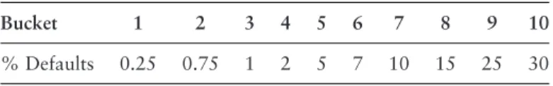
The value of the log-rank Q statistic for benchmarking both rating systems is 15.91, well above the critical value of 3.84 at a 5% confidence level, rejecting the null hypothesis of equivalence of the two benchmarked rating systems ( Table 7.4).
Credible mapping
- The mapping process
- An empirical illustration
In addition, each risk class level k in subportfolio j is also assumed to be characterized by an unobservable risk parameter jk. In effect, the calculation reduces to a second-stage estimation of the standard credibility factor on the resulting 10-bucket mapped rating scale and corresponding portfolio. As before, the specific Gamma-Poisson model underlying Model 1 allows the use of Equation 7.11 to directly derive new credibility estimates for the mapped rating scale.
The resulting mapped rating scale and the corresponding authentic ratings can now be compared to the reference rating scale.
Further elements of modern credibility theory
Studies on the Validation of Internal Rating Systems, Basel Committee Working Paper, 14 May. 2006) Plausibility Estimators in Multiplicative Models, Research Report 3. 1980).
Proof of the credibility fundamental relation
Under Assumptions 1 and 2, the best linear (non-homogeneous) estimator (Bühlmann, 1967) of the expected risk for class k conditional on the risk driver is . Test One seeks the best linear approximation of "k, the risk of class k with the risk driver. 34;k, from a random variable W = Cr "k assumed to be an affine combination of all observations Zij of the entire portfolio .
Wis therefore the orthogonal projection of the "con subspace spanned by the random variables (1 Zij).
Mixed Gamma–Poisson distribution and negative binomial
Calculation of the Bühlmann credibility estimate under the Gamma–Poisson model
Calculation of accuracy ratio
8 Analytic models of the ROC Curve
- Theoretical implications and applications
- The validation of credit rating system
- CAP and AR
- ROC and the AUROC curve
- Some further statistical properties of ROC measures
- Choices of distributions
- Weibull distribution
- for the two-parameter Weibull model
- for the two-parameter Weibull model
- Logistic distribution
- Normal distribution
- Mixed models
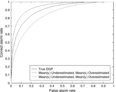
- Performance evaluation on the AUROC estimation with simulated data
- Summary
Engelmannet co. (2003) show that AR is a linear transformation of AUROC; their work complements that of Sobehart and Keenan (2001) with more statistical analysis of the ROC. We then compare the accuracy of the AUROC and CI estimation of the two approaches. In Tables N1–N6, all mean CI widths show that the analytical approach estimates are better than the nonparametric estimates.
In Tables E1 through E6, all the mean absolute errors and the mean CI widths show that the analytic approximation estimates are better than the nonparametric estimates.
Note
The properties of AUROC for normally distributed sample
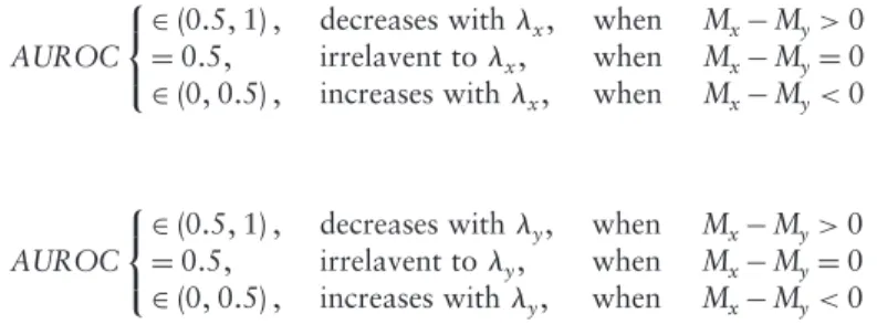
The closer a rating system's AUROC is to 0.5, the less discriminatory power it has. The closer a rating system's AUROC is to 0 or 1, the better its discriminatory power. Therefore, under the assumption of normally distributed scoring variables, the smaller the variance, the better the discriminative power of the rating system.
So, even the discriminative power is higher when we have smaller deviations on X and Y in this case, but the AUROC will be smaller.
9 The validation of equity portfolio risk models
- Linear factor models
- Building a time series model
- Building a statistical factor model
- Definitions
- Principal components
- Building models with known beta’s
- Forecast construction and evaluation
- Diagnostics
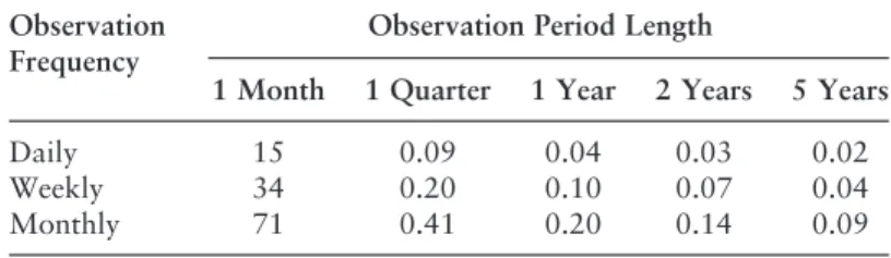
- Time horizons and data frequency
- The residuals
- Monte Carlo procedures
- Conclusions
Indeed, different risk models can be interpreted as different predictions of the same covariance matrix. This is a standard assumption in statistical theory, but we need to think about the realities of the situation. An important issue, not clearly stated by many vendors of risk models, is the time horizon of risk forecasting.
Closely related to the time horizon of the forecast is the frequency of the model.
10 Dynamic risk analysis and risk model evaluation
Volatility over time and the cumulative variance
- Theoretical background
- Explorative approach
- Practical application for portfolio total and active risk
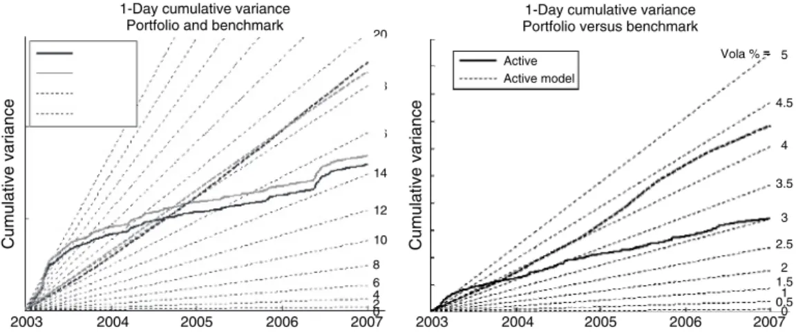
With time measured in years, the slope of the cumulative variance over the time period up to T is equal to the conventional estimate of the variance under the assumption of zero mean. How large is the deviation of the realized cumulative variance relative to the underlying cumulative variance curve. The realized cumulative variance based on the 5-day overlapping data also shows the true underlying cumulative variance.
Comparison with Figure 10.5 nicely demonstrates the advantage of the concept of cumulative variance.
Beta over time and cumulative covariance
- Theoretical Background
- Explorative approach
- Practical application for portfolio beta
This means that the conditional expectation of the realized beta given the benchmark returns is a weighted average of the betas. The conditional variance of the realized beta given the benchmark returns can be derived as. By definition, realized beta is the ratio of the cumulative covariance of the portfolio (or asset) versus the benchmark (or the market) and the benchmark (or market) cumulative variance.
However, for the weekly data sample on the right side of Figure 10.9, the effect of this time scale can be clearly seen as the random fluctuation of the measure cumulative variance becomes larger.
Dynamic risk model evaluation
- Theoretical background
- Realized versus forecast cumulative variance
- Realized versus forecast cumulative beta
- Cumulative variance of forecast-standardized returns
Looking at the same European portfolio using the same long-term risk model, Figure 10.15 shows the cumulative realized and predicted active beta on the left and the predicted risk model active beta on the right. Our second approach for judging the performance or potential bias of a risk model is to look at the cumulative variance of the standardized returns where there is standardization. Figure 10.16 on the left shows again the European portfolio with daily data using the long-term risk model to standardize returns.
In May 2006, the slope was 1.4, and the model underestimated the risk in this period accordingly.
11 Validation of internal rating systems and PD estimates ∗
- Regulatory background
- Statistical background
- Conceptual considerations
- Basic setting
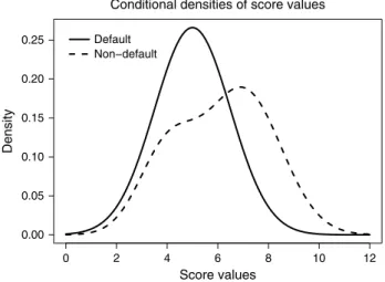
- Describing the joint distribution of (S,Z) with conditional densities
- Describing the joint distribution of (S,Z) with conditional PDs
- Equivalence of the both descriptions
- A comment on conditional PDs
- Dealing with cyclical effects
- The situation in practice
- Mapping score values on rating grades
- Monotonicity of conditional PDs
- Cut-off decision rules
- Conclusions for practical applications
- Discriminatory power of rating systems
- Cumulative accuracy profile
- Accuracy ratio
- Receiver operating characteristic
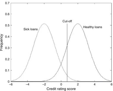
In such a situation, Bayes' formula is useful to derive the conditional PDs given the values of the score variable. Assume further that the conditional PD, P[DS=s], as a function of the score values is decreasing in its arguments. Are there any reasonable conditions such that the monotonicity of the conditional PDs given the score is guaranteed.
Another closely related way of characterization is by means of the conditional probability of default given the outcome values.