A Generative Deep Learning Approach for Shape Recognition of Arbitrary Objects from Phaseless Acoustic Scattering Data

A Generative Deep Learning Approach for Shape Recognition of Arbitrary Objects from Phaseless Acoustic Scattering Data

Item Type Article

Authors Ahmed, Waqas Waseem;Farhat, Mohamed;Chen, Pai-Yen;Zhang, Xiangliang;Wu, Ying

Citation Ahmed, W. W., Farhat, M., Chen, P.-Y., Zhang, X., & Wu, Y. (2023).

A Generative Deep Learning Approach for Shape Recognition of Arbitrary Objects from Phaseless Acoustic Scattering Data.

Advanced Intelligent Systems, 2200260. Portico. https://

doi.org/10.1002/aisy.202200260 Eprint version Publisher's Version/PDF

DOI 10.1002/aisy.202200260

Publisher Wiley

Journal Advanced Intelligent Systems

Rights Archived with thanks to Advanced Intelligent Systems under a Creative Commons license, details at: http://

creativecommons.org/licenses/by/4.0/

Download date 2024-01-01 17:19:16

Item License http://creativecommons.org/licenses/by/4.0/

Link to Item http://hdl.handle.net/10754/679785

Supplementary Information

A Generative deep learning approach for shape recognition of arbitrary objects from phaseless acoustic scattering data

Waqas W. Ahmed¹, Mohamed Farhat¹, Pai-Yen Chen², Xiangliang Zhang^1,3†, and Ying Wu^1,4*

1Division of Computer, Electrical and Mathematical Sciences and Engineering, King Abdullah University of Science and Technology (KAUST), Thuwal, 23955-6900, Saudi Arabia

2Department of Electrical and Computer Engineering, University of Illinois at Chicago, Chicago, IL60607, United States of America

3Department of Computer Science and Engineering, University of Notre Dame, Notre Dame, IN 46556, United States of America

4Division of Physical Sciences and Engineering, King Abdullah University of Science and Technology (KAUST), Thuwal, 23955-6900, Saudi Arabia

Emails: ^*ying.wu@kaust.edu.sa, ^†xzhang33@nd.edu

This supplementary information contains details on the analytic formula of acoustic wave scattering by solid objects derived from Mie scattering, which is used to validate the numerical simulations performed using COMSOL Multiphysics to generate the scattering data(Section 1)； the definition of the structure similarity index measure (SSIM) (Section 2); the analysis of the effect of number of frequencies on the object detection (Section 3); the effect of a half-plane far- field data (Section 4); and more examples for reconstruction of arbitrary objects (Section 5).

1. Validation of numerical simulation of acoustic scattering by solid scatterers

Let us consider the elastic cylinder shown in Fig. S1, with radius 𝑎, density 𝜌₁, and speeds of sound 𝑐₁ and 𝑐₂ , corresponding to pressure (longitudinal) and shear (transverse) waves, respectively.

Fig. S1. Scheme and geometry of the acoustic wave scattering from an infinitely extended (in the 𝑧 −direction) elastic cylinder.

1.1 General governing equations

The general (linear) equation governing the propagation of elastic waves in solids (taking into account shear waves) is given by

(𝜆 + 2𝜇)∇(𝜍) − 𝜇∇ × (2𝛀) = 𝜌₁𝜕²𝒖

𝜕𝑡², (1.1) with 𝜍 = ∇ ∙ 𝒖 and 2𝛀 = ∇ × 𝒖. From Eq. (1.1) we can derive the equations for 𝜍 and 2𝛀 as

∆𝜍 = 𝜌₁ 𝜕²𝜍

, (1.2)

and

∆(2𝛀) =𝜌₁ 𝜇

𝜕²(2𝛀)

𝜕𝑡² , (1.3)

where the velocities can be defined as

𝑐₁ = √𝜆 + 2𝜇

𝜌₁ ; 𝑐₂ = √𝜇

𝜌₁, (1.4)

where 𝜆 and 𝜇 are the Lamé parameters.

In order to solve Eq. (1.1) we need to rewrite the displacement vector as

𝒖 = −∇𝜓 + ∇ × 𝑨, (1.5)

to obtain

∆𝜓 = 1 𝑐₁²

𝜕²𝜓

𝜕𝑡² and ∆𝑨 = 1 𝑐₂²

𝜕²𝑨

𝜕𝑡² (1.6)

To solve Eq. (1.6) in the case of cylindrical objects (Fig. S1) we can use the following ansatz

𝜓 = ∑ 𝑎_𝑛𝐽_𝑛(𝑘₁𝑟) cos 𝑛𝜃

∞

𝑛=0

, (1.7)

𝐴_𝑧 = ∑ 𝑏_𝑛𝐽_𝑛(𝑘₂𝑟) sin 𝑛𝜃

∞

𝑛=0

, (1.8)

with the wavenumbers 𝑘_𝑖 = 𝜔/𝑐_𝑖. Equation (1.8) is shown to be valid as 𝑨 can be shown to have components in the 𝑧-direction because of symmetry considerations. Also, only sin𝑛𝜃 terms appear in Eq. (1.8) as the potential vector has to be anti-symmetrical about the axis 𝜃 = 0, to ensure that the resulted displacement is symmetrical around 𝜃 = 0.

Therefore, by combining Eq. (1.5) and Eqs. (1.7)-(1.8), we can get

𝑢_𝑟 = ∑ {𝑛𝑏_𝑛

𝑟 𝐽_𝑛(𝑘₂𝑟) − 𝑎_𝑛 𝑑

𝑑𝑟𝐽_𝑛(𝑘₁𝑟)} cos 𝑛𝜃

∞

𝑛=0

, (1.9)

𝑢_𝜃 = ∑ {𝑛𝑎_𝑛

𝑟 𝐽_𝑛(𝑘₁𝑟) − 𝑏_𝑛 𝑑

𝑑𝑟𝐽_𝑛(𝑘₂𝑟)} sin 𝑛𝜃

∞

𝑛=0

. (1.10)

On the other hand, the incident plane wave can be represented by 𝑝_𝑖 = 𝑃₀𝑒^{−𝑖𝑘3𝑥} = 𝑃₀𝑒^{−𝑖𝑘3𝑟cos𝜃} = 𝑃₀∑ 𝜀_𝑛(−𝑖)^𝑛𝐽_𝑛(𝑘₃𝑟) cos 𝑛𝜃

∞

𝑛=0

. (1.11)

where 𝜀₀ = 1 and 𝜀_𝑛≥1= 2. The radial component of the displacement of this incident plane wave is thus (from now on we assume, without loss of generality, that 𝑃₀ = 1 to simplify the expressions)

𝑢_𝑖,𝑟= 1 𝜌₃𝜔²

𝜕𝑝_𝑖

𝜕𝑟 = 1

𝜌₃𝜔²∑ 𝜀_𝑛(−𝑖)^𝑛 𝑑

𝑑𝑟𝐽_𝑛(𝑘₃𝑟) cos 𝑛𝜃

∞

𝑛=0

, (1.12)

and the scattered wave is

𝑝_𝑠 = ∑ 𝑐_𝑛𝐻_𝑛⁽¹⁾(𝑘₃𝑟) cos 𝑛𝜃

∞

𝑛=0

, (1.13)

and its associated radial component of displacement is

𝑢_𝑠,𝑟 = 1

𝜌₃𝜔²∑ 𝑐_𝑛 𝑑

𝑑𝑟𝐻_𝑛⁽¹⁾(𝑘₃𝑟) cos 𝑛𝜃

∞

𝑛=0

, (1.14)

where 𝑐_𝑛 are the scattering coefficients, to be evaluated via the boundary conditions of the problem, along with the coefficients 𝑎_𝑛 and 𝑏_𝑛.

1.2 Boundary conditions and numerical simulations

In the case of an elastic cylinder in an acoustical media (such as water) the boundary conditions that shall be employed on the cylinder’s boundaries are: (i) The pressure in the fluid must be equal to the normal component of stress at the solid interface; (ii) the radial component of displacement of the fluid has to be equal to the normal component of displacement of the solid interface; and (iii) the tangential components of shear stress must vanish at the interface of the solid. This means specifically

𝑝_𝑖+ 𝑝_𝑠 = −[𝑟𝑟] at 𝑟 = 𝑎, (1.15)

𝑢_𝑖,𝑟 + 𝑢_𝑠,𝑟 = 𝑢_𝑟 at 𝑟 = 𝑎, (1.16)

[𝑟𝜃] = [𝑟𝑧] = 0 at 𝑟 = 𝑎, (1.17)

where the stress components in cylindrical coordinates are [𝑟𝑟] = 𝜆𝜍 + 2𝜇𝜕𝑢_𝑟

𝜕𝑟 = 2𝜌₁𝑐₂²{(𝜎𝕀 − 2𝜎)𝜍 +𝜕𝑢_𝑟

𝜕𝑟}, (1.18)

[𝑟𝜃] = 𝜇 {1 𝑟

𝜕𝑢_𝑟

𝜕𝜃 + 𝑟 𝜕

𝜕𝑟(𝑢_𝜃

𝑟 )}, (1.19)

[𝑟𝑧] = 𝜇 {𝜕𝑢_𝑟

𝜕𝑧 +𝜕𝑢_𝑧

𝜕𝑟}. (1.20)

By applying the boundary conditions at the interface between the elastic cylinder and the surrounding fluid, we get the linear system

(

−𝑥₁𝐽_𝑛^′(𝑥₁) 𝑛𝐽_𝑛(𝑥₂) ^−𝑥3

𝜌3𝜔²𝐻_𝑛^(1)′(𝑥₃) 𝑥₁²[−2𝜇𝐽_𝑛^′′(𝑥₁) + 𝜆𝐽_𝑛(𝑥₁)] 2𝜇𝑛[𝑥₂𝐽_𝑛^′(𝑥₂) − 𝐽_𝑛(𝑥₂)] 𝑎²𝐻_𝑛⁽¹⁾(𝑥₃)

2𝑛[𝑥₁𝐽_𝑛^′(𝑥₁) − 𝐽_𝑛(𝑥₁)] −𝑛²𝐽_𝑛(𝑥₂) + 𝑥₂𝐽_𝑛^′(𝑥₂) − 𝑥₂²𝐽_𝑛^′′(𝑥₂) 0

) ( 𝑎_𝑛 𝑏_𝑛 𝑐_𝑛

) =

( 𝑥₃

𝜌₃𝜔²𝐽_𝑛^′(𝑥₃)

−𝑎²𝐽_𝑛(𝑥₃) 0

). (1.21)

where 𝑥_𝑖 = 𝑘_𝑖𝑎.

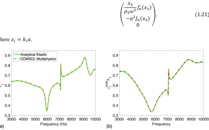
Fig. S2. Scattering cross-section (SCS) from an elastic cylinder made of (a) steel and (b) Aluminum embedded inside water. The dashed (red) curve gives the COMSOL simulations whereas the green solid curves give the Mie results discussed in this section.

To obtain 𝑐_𝑛 we make use of the Cramer’s rule, i.e., 𝑐_𝑛 = ^{det 𝑉𝑛}

det 𝑀𝑛, where 𝑀_𝑛 is the matrix appearing in the LHS of Eq. (1.21) and 𝑉_𝑛 is the matrix obtained from 𝑀_𝑛 by replacing its last column by the RHS of Eq. (1.21).

In order to verify the validity of the COMSOL Multiphysics elastic/acoustic modeling of scattering, we compute and give in Fig. S2 the SCS of a cylinder by using both COMSOL (red dashed lines) and the Mie formalism discussed in the previous paragraphs (green solid lines).

These results match perfectly for both a steel cylinder of radius 20 cm [Fig. S2(a)] in water and an

Aluminum cylinder [Fig. S2(b)] in water, validating thus the numerical modeling by COMSOL, that we use throughout this paper.

2. Structure Similarity Index Measure (SSIM)

SSIM is a metric that quantify the similarity between two given images by extracting key characteristic from an image named Luminance, Contrast, and Structure. Luminance is measured by averaging over all the pixel value denoted by 𝜇 reads as: 𝜇_𝑥= ¹

𝑁∑^𝑁_𝑖=0𝑥_𝑖. Contrast is measured by taking the standard deviation of all the pixel values denoted by σ reads as: 𝜎_𝑥 =

√ ¹

𝑁−1∑^𝑁_𝑖=0(𝑥_𝑖 − 𝜇_𝑥)² and structure comparison is computed by (𝑥 − 𝜇_𝑥) 𝜎⁄ _𝑥. The luminance comparison function 𝑙(𝑥, 𝑦) is a function of 𝜇_𝑥 and 𝜇_𝑦 defined as:

𝑙(𝑥, 𝑦) = 2𝜇_𝑥𝜇_𝑦+ 𝑐₁ 𝜇_𝑥² + 𝜇_𝑦² + 𝑐₁

The contrast comparison function 𝑐(𝑥, 𝑦) is a function of 𝜎_𝑥 and 𝜎_𝑥 defined as:

𝑐(𝑥, 𝑦) = 2𝜎_𝑥𝜎_𝑦+ 𝑐₂ 𝜎_𝑥²+ 𝜎_𝑦²+ 𝑐₂

Structure comparison function 𝑠(𝑥, 𝑦)is defined as:

𝑠(𝑥, 𝑦) =2𝜎_𝑥𝑦+ 𝑐₃ 𝜎_𝑥𝜎_𝑦+ 𝑐₃

where 𝜎_𝑥𝑦= √ ¹

𝑁−1∑^𝑁_𝑖=0(𝑥_𝑖 − 𝜇_𝑥)²(𝑦_𝑖− 𝜇_𝑦)², and 𝑐₁, 𝑐₂, 𝑐₃ are constants to ensure stability when the denominator becomes 0.

And finally, luminance, contrast, and structure comparison functions are combined to determine the similarity index value given by,

SSIM(𝑥, 𝑦) = [𝑙(𝑥, 𝑦)]^𝛼[𝑐(𝑥, 𝑦)]^𝛽[𝑠(𝑥, 𝑦)]^𝛾

where 𝛼 > 0, 𝛽 > 0, 𝛾 > 0 denote the relative strength of each of the metrics. To simplify the expression, we assume, 𝛼 = 𝛽 = 𝛾 = 1 and 𝑐₃ = 𝑐₂/2 that results in:

SSIM(𝑥, 𝑦) = (2𝜇_𝑥𝜇_𝑦+ 𝑐₁)(2𝜎_𝑥𝑦+ 𝑐₂) (𝜇_𝑥²+ 𝜇_𝑦²+ 𝑐₂)(𝜎_𝑥²+ 𝜎_𝑦²+ 𝑐₂)

We used SSIM to determine the quality of the reconstructed and generated objects in the main text.

3. Object detection from Single to multifrequency far-field radiation data

In the main text, we presented the results for five frequencies radiation data to determine the shape of object accurately. By including multifrequency data in the training process, we demonstrate how the results are significantly improved by providing training and prediction of neural networks with different frequencies.

3.1 Object detection from Single frequency far-field radiation profile

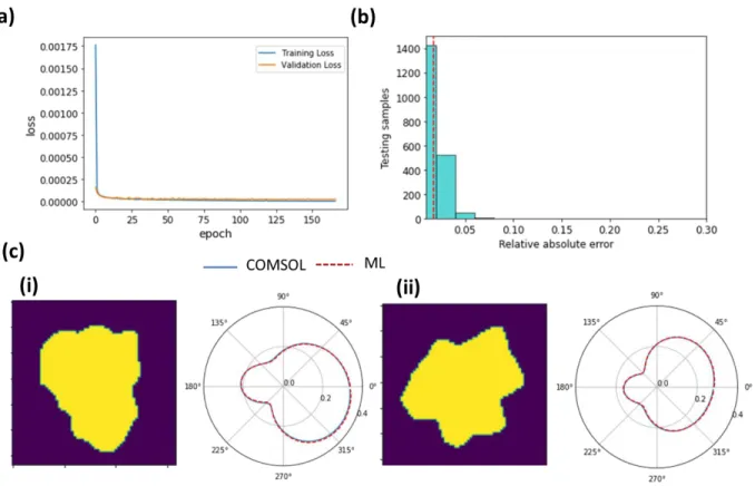
We start our analysis with a single frequency (𝑓₁= 1 kHz) radiation data and designed the neural network to solve the forward and inverse problem. The five-layer forward neural network is designed containing 4096 − 500 − 500 − 500− 400 − 400 −87 nodes. The LeakyReLu function is used for activation, and Adam optimization is used with a learning rate 10⁻⁴. The training and prediction results for the designed forward network are shown in Figs. S3(a) and S3(b), respectively. The relative prediction error is computed over the testing data with mean error 0.0172 indicated by vertical red dashed line. Fig. S3(c) illustrates the comparison of computed

radiation pattens for two given arbitary objects where the COMSOL results (solid blue curve) are in perfect agreement with ML predictions (red dashed curve).

Fig. S3. Training and prediction performance of forward designed neural network for single frequency far- field radiation data. (a) Learning curve of optimized network. (b) Histogram of spectral prediction error.

(c) Representative examples for far-field prediction from given arbitary objects. The solid blue and dotted red line represent the far-field response calculated from COMSOL and ML method, respectively.

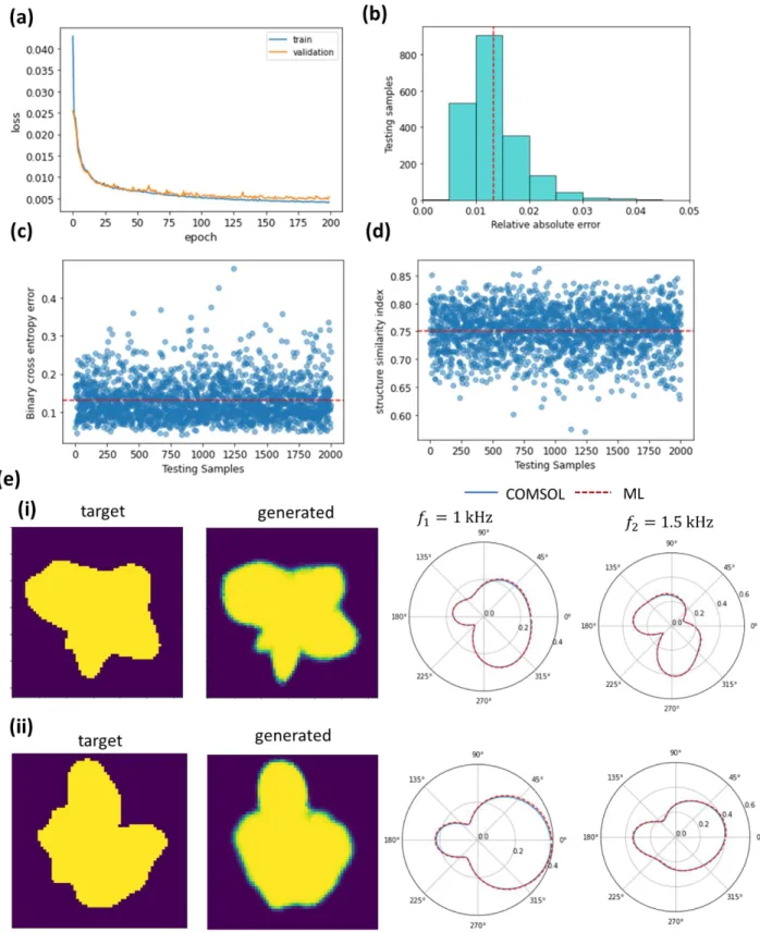
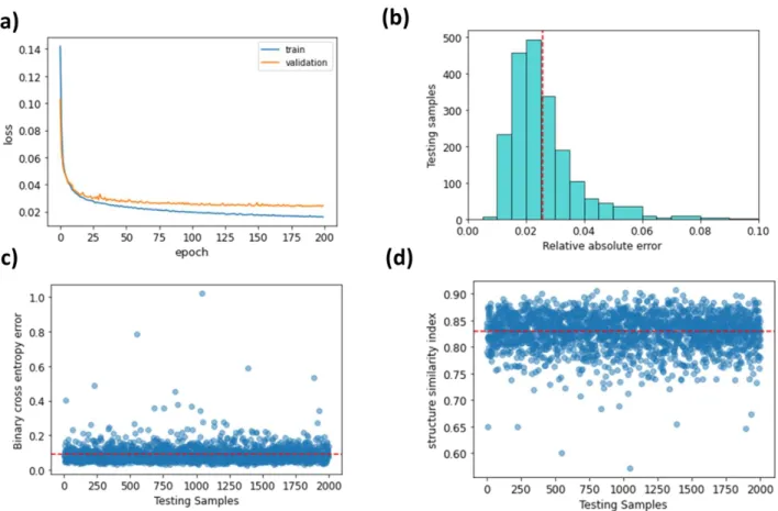
Next, we proceed to solve the inverse problem of arbitary shape detection with single frequency far-field data. The inverse designed network contains 87− 800 − 500 − 500− 500 − 400 −100 nodes. The training and prediction results are presented in Fig.S4. The relative spectral error, binary cross-entropy error (BCE) and SSIM over generated objects for the testing data are computed with mean values of 0.007, 0.271, and 0.70 respectively. Although the spectral error is

very low but large BCN error in generated geometries as compared to target objects is expected due to presence of non-unique solution space, as depicted in Fig. S4(e).

Fig. S4. Training and prediction performance of inverse designed neural network for single frequency far- field radiation data. a Learning curve of optimized network. (b) Histogram of spectral prediction error. (c) binary cross-entropy error for ML generated shapes. (d) distribution of SSIM for the ML generated geometries. (e) Representative examples for arbitrary object prediction from given one-frequency far-field data. The predicted far-field response (dashed red) from the generated objects exactly matches with (solid blue) but the generated shapes show variations from the target objects due to non-unique solution space in inverse process.

3.2 Object detection from far-field radiation profile at two different frequencies

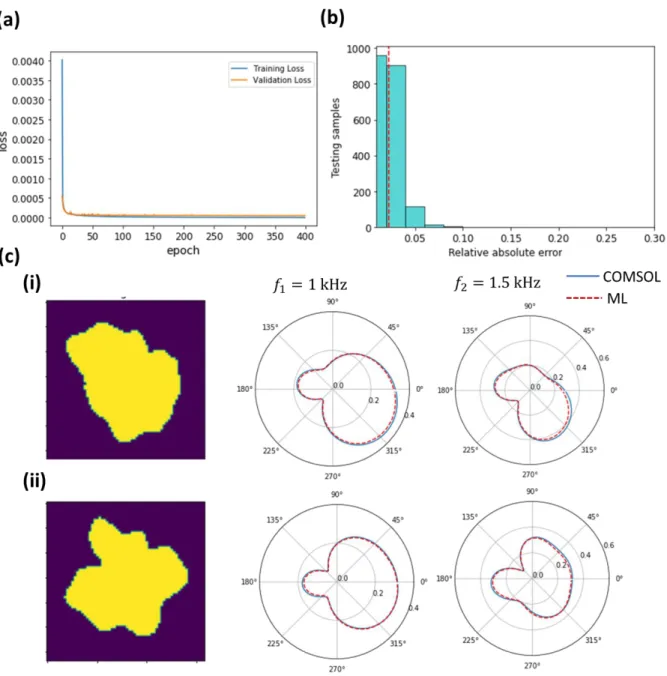
Next, we train the network with far-field radiation data at two different frequencies 𝑓₁ = 1 kHz and 𝑓₂ = 1.5 kHz. The forward and inverse architectures consist of 4096 − 500 − 500 − 500− 400

− 174 and 174− 800 − 800 − 500 − 500− 500 − 400 −100 nodes, respectively. The training and prediction results for forward and inverse network are shown in Figs. S5 and S6, respectively. On Fig.S5(b), the red line indicates the mean relative spectral error for trained forward network as 0.0227. In inverse network, the relative spectral error, binary cross-entropy error (BCE) and SSIM over generated objects for the testing data are computed with mean values of 0.0135, 0.131, and 0.75 respectively, as depicted in Fig.S6.

Fig. S5. Training and prediction performance of forward designed neural network for far-field radiation data at two different frequencies. (a) Learning curve of optimized network. (b) Histogram of spectral prediction error. (c) Representative examples for far-field prediction from given arbitrary objects. The solid blue and dotted red line represent the far-field response calculated from COMSOL and ML method, respectively.

Fig. S6 Training and prediction performance of inverse designed neural network for two-frequency far- field radiation data. (a) Learning curve of optimized network. (b) Histogram of spectral prediction error.

(c) binary cross-entropy error for ML generated shapes. (d) distribution of SSIM for the ML generated geometries. (e) Representative examples of arbitrary object prediction from given two-frequency far-field data. The predicted far-field response (dashed red) from the generated objects exactly matches with (solid blue) but the generated shapes show variations from the target objects due to non-unique solution space in inverse process.

3.3 Object detection from far-field radiation profile at three different frequencies

Subsequently, we consider three different frequencies 𝑓₁ = 1 kHz 𝑓₂ = 1.5 kHz, and 𝑓₃= 2 kHz. The results for the trained forward and inverse networks are shown in Figs. S7 and S8, respectively.

The designed forward and inverse architectures consist of 4096 − 500 − 500 − 500− 400 − 400

−261 and 174− 800 − 800 − 500 − 500− 500 − 400 −100 nodes, respectively. The red dashed line in Fig. S7(b) indicates the mean relative spectral error for the trained forward network as 0.027.

For the inverse case, relative spectral error, binary cross-entropy error (BCE), and SSIM over generated objects are computed with mean values of 0.0196, 0.0986, and 0.79, respectively [see Fig.S8].

Fig. S7. Training and prediction performance of forward designed neural network for far-field radiation data at three different frequencies. (a) Learning curve of optimized network. (b) Histogram of spectral prediction error. (c) Representative examples for far-field prediction from given arbitrary objects. The solid blue and dotted red line represent the far-field response calculated from COMSOL and ML method, respectively.

Fig. S8 Training and prediction performance of inverse designed neural network for far-field radiation data at three different frequencies. (a) Learning curve of optimized network. (b) Histogram of spectral prediction error. (c) binary cross-entropy error for ML generated shapes. (d) Distribution of SSIM for the ML generated geometries (e) Representative example arbitrary object prediction from given three-frequency far-field data. The predicted far-field response (dashed red) from the generated objects exactly matches with (solid blue) but the generated shapes show variations from the target objects due to non-unique solution space in inverse process. The results of arbitrary shape detection are significantly improved due to addition of extra information in the training process as compared to Figs.S5 and S6.

3.4 Object detection from far-field radiation profile at four different frequencies

Lastly, we train the network with far-field radiation data at four different frequencies 𝑓₁= 1 kHz 𝑓₂ = 1.5 kHz, 𝑓3= 2 kHz and 𝑓4= 2.5 kHz and results for trained forward and inverse networks are presented in Figs. S9 and S10, respectively. The designed forward and inverse architectures consist of –4096 – 800 – 800 − 800– 800 − 600 −600−348 and 348– 800 – 800 – 500 − 500– 500 − 400

−100 nodes, respectively. Fig. S(9) illustrates the distribution of relative spectral error over testing data with mean value 0.0313. Fig. S10 shows the inverse network's relative spectral error, binary cross-entropy error (BCE) and SSIM over the generated objects with mean values of 0.025, 0.0916, and 0.83 respectively.

Fig. S9. Training and prediction performance of forward designed neural network for far-field radiation data at four different frequencies. (a) Learning curve of optimized network. (b) Histogram of spectral

blue and dotted red line represent the far-field response calculated from COMSOL and ML method, respectively.

Fig. S10. Training and prediction performance of inverse designed neural network for far-field radiation data at four different frequencies. (a) Learning curve of optimized network. (b) Histogram of spectral prediction error. (c) binary cross-entropy error for ML generated shapes. d distribution of SSIM for the ML generated geometries.

4. Object detection from multifrequency half-plane far-field data

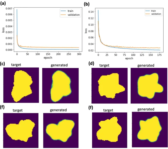
Here, we present the training behavior of designed neural network to predict the shape of arbitary object from multifrequency half-plane far-field data which is discussed in the main text. The designed forward and inverse architectures consist of 4096 − 1000 − 1000 − 800− 800 − 600 −600

−328 and 328− 800 − 800 − 500 − 500− 400 −100 nodes, respectively. In addition, some more examples are provided for arbitary shape detection from the given far-field patterns.

Fig. S11. Training performance of designed neural network for half- plane multifrequency far-field radiation data. (a) Learning curve of forward optimized network. (b) Learning curve of inverse optimized network. (c-f) target object and generated object from the inverse designed network.

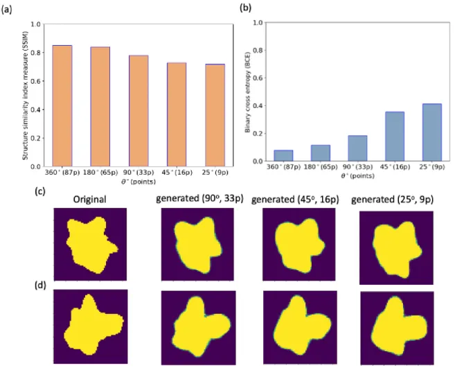
5. Effect of sampling and angular interval on the detection efficiency

In order to analyze the effect of sampling rate on the recognition process, we perform the following two sets of studies. In the first set, we keep the angular range unchanged but reduce the number of

range. For the first three cases (87,29, and 9) the structure similarity index measure (SSIM) remains almost unchanged as shown in Fig. S12(a). The binary cross entropy (BCE) displays similar behavior (Fig. S12(b)). This shows that the recognition mechanism works well for certain number of reduced sampling points. In order to further showcase this point, we show in Figs. S12(c)-(d) the shape recognition mechanism for two random shapes, with both 29 and 9 sampling points where the generated shape reconstructs well the original one. Only when the sampling number of points is reduced to 3, deterioration of the shape is observed in the rightmost panel of Figs. S12(c) and (d). The SSIM and the BCE depart quite largely from the other scenarios.

Fig. S12. (a) structure similarity index measure and (b) binary cross entropy, for different sampling points.

(c)-(d) show the original and the generated shape for 29, 9, and 3 sampling points for two objects.

In the second set, we reduce both the sampling number of points as well as the angular range.

Specifically, we consider 360 degrees, 180 degrees, as well as 90 degrees, 45 and 25 degrees, with 87, 65, 33, 16 and 9 sampling points, respectively. The results over the testing data are shown in Fig. S13. As we reduce the angular range with sampling points, the efficacy of the model to determine the unique shape decreases due to less spectral information.

Fig. S13. (a) Structure similarity index measure and (b) binary cross entropy, for different angular intervals.

(c)-(d) Original and generated shape for 90^o (33 points), 45^o (16 points), and 25^o (9 points) angular interval, for two different objects.

To conclude, fewer sampling points would not significantly affect the recognition performance as long as the number of sampling points and the angular coverage are above certain threshold.

6. More examples for reconstruction of arbitrary Object from AAE

Here, we present some more examples to reconstruct the arbitrary object from the designed AAE in the main text.

Fig. S14. Examples of object reconstruction from trained adversarial autoencoder discussed in main text.