1-Modes of heat transfer (conduction, convection & radiation) 2-Thermal resistances

1

Summary of correlations, figures and tables for MEP460 Heat Exchanger Design

1-Modes of heat transfer (conduction, convection & radiation) 2-Thermal resistances

3-Fins (fin efficiency 𝜂

_𝑓

, overall surface efficiency 𝜂

_𝑜

) 4-Fouling

5-Overal heat transfer coefficient, U 6-Pressure drop (major and minor losses) 7-Dimensionless numbers

8-Correlations for external convective heat transfer flows 9-Correlations for internal convective heat transfer flows 10-Corelations for free convective heat transfer

11-Corelations for boiling heat transfer

12-Correlations for condensation heat transfer

13-Heat exchanger LMTD and Effectiveness-NTU relations and figures 14-Compact Heat Exchangers

15-Summary of Ch.3 & Ch. 4 from Kakac book 16-Double pipe heat exchangers

17-Shell and tube heat exchangers-Kern method

18- Shell and tube heat exchangers-Dell & Delaware method

19-Typical values for shell and tube heat exchanger parameters

20-Cooling Towers

2

1-Modes of heat transfer

𝑞 = −𝑘𝐴 𝑑𝑇

𝑑𝑥 𝑞 = ℎ𝐴(𝑇

_𝑠

− 𝑇

_∞

) ^𝑞

𝑔𝑟𝑎𝑦

= 𝜖𝜎𝑇

⁴

2-Thermal resistances

Plain Wall Cylindrical system

𝑅_𝑤= 𝐿 𝑘𝐴⁄ 𝑅_𝑤= ln(𝑟₂⁄ ) 2𝜋𝑘𝐿𝑟₁ ⁄

3-Fins

One way to increase heat transfer form a surface is by increasing the heat transfer area

𝑞

_𝑐

= ℎ𝐴(𝑇

_𝑠

− 𝑇

_∞

)

3

straight uniform section fins Increase heat transfer by adding fins to the surface

Circular (annular) fins on circular tubes pin fins

Most common fins are straight fin on plain surface and circular fins on circular tube

4

3.1 Fin Efficiency 𝜼

_𝒇

𝜂

_𝑓

= 𝑞

_𝑓

𝑞

_𝑚𝑎𝑥

= 𝑞

_𝑓

ℎ𝐴

_𝑓

𝜃

_𝑏

𝑞

_𝑓

= 𝜂

_𝑓

𝑞

_𝑚𝑎𝑥

= 𝜂

_𝑓

ℎ𝐴

_𝑓

𝜃

_𝑏

𝜃

_𝑏

= (𝑇

_𝑏

− 𝑇

_∞

) T

b

is the base or wall temperature, A

f

is the fin area.

a) For straight fin of uniform cross-section or pin fin, the fin efficiency is given by 𝜂

_𝑓

= tanh (𝑚𝐿)

𝑚𝐿

𝑚 = √ℎ𝑃 𝑘𝐴_𝑐

P is the perimeter (=D for pin fin), A

_c

is the cross-section area of the fin)

Efficiency of straight fins Efficiency for circular (annular) fins in circular tubes

continuous fins on circular Continuous fins on circular pipe Continuous fins on flat tubes

5

pipe (in-lined arrangement) (staggered arrangement)

Approximate fin efficiency for circular (annular) fin on circular pipe 𝜂_𝑓 =tanh (𝑚𝜙𝑟₁)

𝑚𝜙𝑟₁

𝑚 = √ 2ℎ 𝑘_𝑓𝛿_𝑓

𝜙 = (𝑟₂⁄𝑟₁− 1)[1 + 0.35ln (𝑟₂⁄ ] 𝑟₁

𝛿_𝑓 is the fin thickness and kf is the thermal conductivity of the material.

For 0.8 < 𝑟₂⁄𝑟₁< 1 and 0.5 < 𝜂_𝑓 < 1 , the error is < 1 %. [Ref. ASHRAE, book of fundamentals]

b) Continuous fins

Fin efficiency for continuous fin on circular tubes[Square array]

𝜂_𝑓=tanh (𝑚𝜙𝑟1) 𝑚𝜙𝑟₁

𝜙 = (𝑟_𝑒⁄𝑟₁− 1)[1 + 0.35 ln (𝑟_𝑒⁄ ] 𝑟₁ 𝑟_𝑒

𝑟₁= 1.28𝜓(𝛽 − 0.2)^0.5 Where (see the figure)

𝜓 = 𝑀 𝑟⁄ ₁, 𝛽 = 𝐿 𝑀⁄ , 𝛽 must be P1. If <1 replace L by M.

Fin efficiency for continuous fin on circular tubes[hexagonal array]

𝜂_𝑓 =tanh (𝑚𝜙𝑟₁) 𝑚𝜙𝑟₁

𝜙 = (𝑟_𝑒⁄𝑟₁− 1)[1 + 0.35 ln (𝑟_𝑒⁄ ] 𝑟₁ Where (see the figure)

𝑟_𝑒⁄𝑟₁= 1.27 𝜓(𝛽 − 0.3)^0.5 𝜓 = 𝑀 𝑟⁄ ₁, 𝛽 = 𝐿 𝑀 ⁄

𝑀 = 𝑆_𝑇⁄2 𝑜𝑟 𝑆_𝐿 𝑤ℎ𝑖𝑐ℎ𝑒𝑣𝑒𝑟 𝑙𝑒𝑠𝑠 𝐿 = 0.5√(𝑆_𝑇⁄ )2 ²+ (𝑆_𝐿)²

Continuous fins on circular pipe [Square array]

Continuous fins on circular tubes [Hexagonal array]

6

7

Fin efficiency for continuous fin on non-circular pipe flat tube (square or staggerd array) 𝜂_𝑓=tanh (𝑚𝑙)

𝑚𝑙

𝑚 = ( 2ℎ 𝑘_𝑓𝛿_𝑓)

1 2⁄

where

h convective heat transfer coefficient [W/(m².K)]

kf thermal conductivity, [W/(m.K)]

𝛿𝑓 fin thickness [m]

𝑙 fin length (𝑆_𝑇− 𝐿_2,𝑜) 2⁄

Continuous fin on flat tube

8

3.2 Surface overall efficiency 𝜼

_𝒐

The heat transfer form a finned surface is given by

𝑞 = 𝑞

_𝑢𝑛

+ 𝑞

_𝑓

= 𝐴

_𝑢𝑓

ℎ𝜃

_𝑏

+ 𝐴

_𝑓

ℎ𝜂

_𝑓

𝜃

_𝑏

𝜃

_𝑏

= 𝑇

_𝑏

− 𝑇

_∞

𝐴 = 𝐴

_𝑓

+ 𝐴

_𝑢𝑓

𝑞 = ((𝐴 − 𝐴

_𝑓

) + 𝜂

_𝑓

𝐴

_𝑓

) ℎ𝜃

_𝑏

= 𝐴ℎ [(1 − 𝐴

_𝑓

𝐴 (1 − 𝜂

_𝑓

)] 𝜃

_𝑏

o

is called the surface overall efficiency

𝜂

_𝑜

= 1 − 𝐴

_𝑓

𝐴 (1 − 𝜂

_𝑓

) 4-Fouling

Fouling is generally defined as the deposition and accumulation of unwanted materials such as scale, algae, suspended solids and insoluble salts on the internal or external surfaces of processing equipment including boilers and heat exchangers

Inside and outside fouling

9

Fouling units

𝑅

_𝑓^′′

= [

^𝑚2𝐾

𝑊

]

Fouling resistance for water m

²

.K/W

10

5-Overal heat transfer coefficient

No fins no fouling

1

𝑈

_𝑜

𝐴

_𝑜

= 1

ℎ

_𝑖

𝐴

_𝑖

+ 𝑅

_𝑤

+ 1 ℎ

_𝑜

𝐴

_𝑜

No fins with fouling

1

𝑈

_𝑜

𝐴

_𝑜

= 1

ℎ

_𝑖

𝐴

_𝑖

+ 𝑅

_𝑓𝑖^′′

𝐴

_𝑖

+ 𝑅

_𝑤

+ 𝑅

_𝑓𝑜^′′

𝐴

_𝑜

+ 1 ℎ

_𝑜

𝐴

_𝑜

With fins and fouling

1

𝑈

_𝑜

𝐴

_𝑜

= 1

ℎ

_𝑖

𝜂

_𝑖

𝐴

_𝑖

+ 𝑅

_𝑓𝑖^′′

𝜂

_𝑖

𝐴

_𝑖

+ 𝑅

_𝑤

+ 𝑅

_𝑓𝑜^′′

𝜂

_𝑜

𝐴

_𝑜

+ 1 ℎ

_𝑜

𝜂

_𝑜

𝐴

_𝑜

𝑅_𝑓𝑖^′′= Fouling resistance for the interior surface [m².K/W]

𝑅_𝑓𝑜^′′ Fouling resistance for the exterior surface [m².K/W]

Rw Wall thermal resistance [K/W]

6-Pressure drop

Modified Bernoulli’s equation

𝑃

₁

+ 1

2 𝜌𝑉

₁²

+ 𝜌𝑔𝑧

₁

= 𝑃

₂

+ 1

2 𝜌𝑉

₂²

+ 𝜌𝑔𝑧

₂

+ Δ𝑃

_𝐿

Δ𝑃

_𝐿

= 𝑓 𝐿

𝐷 𝜌𝑉

₂²

+ ∑ 𝐾 𝜌𝑉

²

The first term in the above equation for the major losses due to wall friction and the second term is for

2

the minor losses due fittings.

11

Friction factor definition

𝑓 = − 𝑑𝑝 𝑑𝑥 ⁄ 𝐷 𝜌𝑢

_𝑚²

⁄ 2

Friction coefficient Cf

𝐶

_𝑓

= 𝜏

_𝑠

𝜌𝑢

_𝑚²

⁄ 2

From the balance of forces for a section of pipe, one can get the relation between the friction factor f and the friction coefficient cf as follows

𝐶

_𝑓

= 𝑓 4

For laminar flow in circular pipe (i.e. Re

_D

<2300 ) 𝑓 =

⁶⁴

𝑅𝑒_𝐷

General turbulent flow in pipes

1

√𝑓 = −2.0 𝑙𝑜𝑔 [ 𝑒 𝐷 ⁄

3.7 + 2.51 𝑅𝑒

_𝐷

√𝑓 ]

Turbulent smooth pipes

𝑓 = (0.79 ∗ 𝑙𝑛𝑅𝑒

_𝐷

− 1.64)

⁻²

e or  is the pipe roughness in meters

12

Moody diagram, Ref. Incropera, 7^th Edition

Pipe roughness, Ref. White, Frank, 5^th Edition

Minor losses due to pipe fittings

Losses due to: (Valves, Elbows, Sudden expansion, Sudden contraction, pipe Entry)

13

Loss coefficient for valves, elbows and tees

Expansion and contraction loss coefficient

14

Friction coefficient for pipe entrances

Boundary layer and entry length

For laminar flor ReD =2300

𝑥_𝑓𝑑,ℎ

𝐷 ≈ 0.05𝑅𝑒_𝐷 For turbulent flow ReD> 2300

10 ≤𝑥_𝑓𝑑,ℎ 𝐷 ≤ 60 Generally it is assumed the flow is fully developed turbulent when

𝑥_𝑓𝑑,ℎ 𝐷 > 10

15

7-Dimensionless numbers

16

17

8-Correlation for external convective heat transfer

18

19

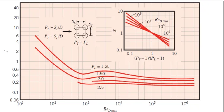
For Aligned arrangement

𝑉

_𝑚𝑎𝑥

= 𝑆

_𝑇

𝑆

_𝑇

− 𝐷 𝑉 𝑅𝑒

_𝑚𝑎𝑥

= 𝜌𝑉

_𝑚𝑎

𝐷

𝜇

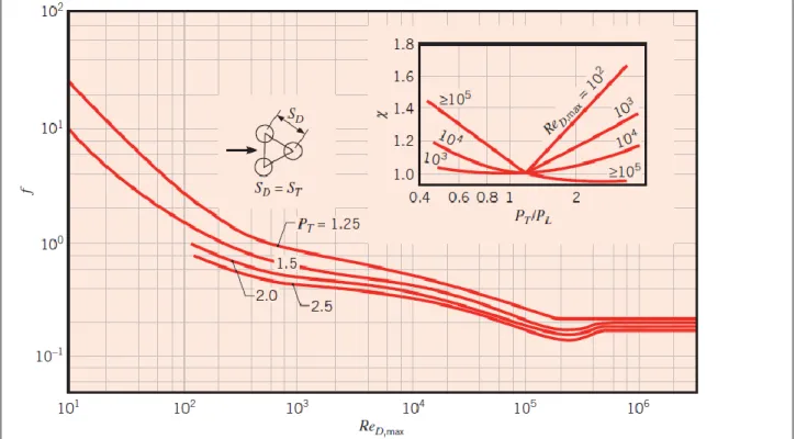
For Staggered arrangement Vmax at A2 if

𝑆

_𝐷

= [𝑆

_𝐿²

+ ( 𝑆

_𝑇

𝑠 )

2

]

1 2⁄

< 𝑆

_𝑇

+ 𝐷 2

then Vmax will be

𝑉

_𝑚𝑎𝑥

= 𝑆

_𝑇

2(𝑆

_𝐷

− 𝐷) 𝑉

Vmax occur at A1

Pressure drop for tube banks

Δ𝑃 = 𝑁

_𝐿

χ (

^{𝜌𝑉𝑚𝑎𝑥}

2

) 𝑓 (7.65)

20

Fig. 7.14 Friction factor ƒ and correction factor  for Equation 7.65. In-line tube arrangement

Fig. 7.15 Friction factor ƒ and correction factor  for Equation 7.65. Staggered tube arrangement

21

9-Correlations for internal convective heat transfer flows

Laminar flows

22

Turbulent Internal Flow

10-Corelations for free (natural) convective heat transfer

Vertical or inclined plates

Properties evaluated at film temperature

𝑇𝑓 =𝑇_𝑠+ 𝑇_∞ 2

Replace g by gcos()

Properties evaluated at film temperature

𝑇_𝑓 =𝑇_𝑠+ 𝑇_∞ 2

 = angle with vertical

0 ≤ 𝜃 ≤ 60

23

Long horizontal cylinder

Sphere

Pr P 0.7 RaD O 10¹¹

24

11-Corelations for boiling heat transfer

Nukiyiama pool boiling curve

Range of 𝚫𝑻

_𝒆

Mode of boiling

Δ𝑇

_𝑒

≤ Δ𝑇

_𝑒,𝐴

Free convection boiling Δ𝑇

_(𝑒,𝐴)

≤ Δ𝑇

_𝑒

< Δ𝑇

_𝑒,𝐶

Nucleate boiling

Δ𝑇

_(𝑒,𝐶)

≤ Δ𝑇

_𝑒

< Δ𝑇

_𝑒,𝐷

Transition Unstable boiling (oscillation between bubble and film boiling)

Δ𝑇

_(𝑒,𝐷)

≤ Δ𝑇

_𝑒

Film Boiling

a) Natural convection

(See Ch. 9 of your textbook) b) Nucleate boiling

Rohsenow formula

𝑞

_𝑠^′′

= 𝜇

_𝑙

ℎ

_𝑓𝑔

[ 𝑔(𝜌

_𝑙

− 𝜌

_𝑣

)

𝜎 ]

1 2⁄

( 𝐶

_𝑝,𝑙

Δ𝑇

_𝑒

𝐶

_𝑠,𝑓

ℎ

_𝑓𝑔

𝑃𝑟

_𝑙^𝑛

)

3

Properties at

T

sat

25

c) Max. heat flux for nucleate boiling

𝑞

_𝑚𝑎𝑥^′′

= 𝐶ℎ

_𝑓𝑔

𝜌

_𝑣

[ 𝜎𝑔(𝜌

_𝑙

− 𝜌

_𝑣

) 𝜌

_𝑣²

]

1 4⁄ C=/24 for horizontal cylinder and spheres C=0.149 for large horizontal plates

Properties at Tsat

d) Min. heat flux (Leidenfrost point)

Leidenfrost point

𝑞

_𝑚𝑖𝑛^′′

= 𝐶𝜌

_𝑣

ℎ

_𝑓𝑔

[ 𝑔𝜎(𝜌

_𝑙

− 𝜌

_𝑣

) (𝜌

_𝑙

+ 𝜌

_𝑣

)

²

]

1 4⁄

C=0.09 Properties at T

_sat

e) Film boiling on horizontal cylinders and spheres

𝑁𝑢 ̅̅̅̅

_𝐷

= ℎ̅

_{𝑐𝑜𝑛𝑣}

𝐷

𝑘

_𝑣

= 𝐶 [ 𝑔(𝜌

_𝑙

− 𝜌

_𝑣

)ℎ

_𝑓𝑔^′

𝐷

³

𝜈

_𝑣

𝑘

_𝑣

(𝑇

_𝑠

− 𝑇

_𝑠𝑎𝑡

) ]

1 4⁄

C=0.62 for horizontal cylinders

C=0.67 for spheres

Properties at

T

_f

except 

_l

and h

fg

at T

sat

26

ℎ

_𝑓𝑔^′

= ℎ

_𝑓𝑔

+ 0.8𝐶

_𝑝,𝑣

(𝑇

_𝑠

− 𝑇

_𝑠𝑎𝑡

)

𝑇

_𝑓

= (𝑇

_𝑠

+ 𝑇

_𝑠𝑎𝑡

) 2 ⁄

ℎ̅

^{4 3⁄}

= ℎ̅

_{𝑐𝑜𝑛𝑣}^{4 3⁄}

+ ℎ̅

_𝑟𝑎𝑑

ℎ̅

^{1 3⁄}

ℎ̅

_𝑟𝑎𝑑

= 𝜖𝜎(𝑇

_𝑠⁴

− 𝑇

_𝑠𝑎𝑡⁴

) 𝑇

_𝑠

− 𝑇

_𝑠𝑎𝑡

If ℎ̅

_𝑟𝑎𝑑

< ℎ̅

_{𝑐𝑜𝑛𝑣}

𝜎 = Stefan-Boltzmann constant =5.67*10

^-8

[W/K

⁴

]

ℎ̅ = ℎ̅

_{𝑐𝑜𝑛𝑣}

+ 3 4 ℎ̅

_𝑟𝑎𝑑

f) Forced Covective boiling

External Flow over a cylinder Low velocity

𝑞

_𝑚𝑎𝑥^′′

𝜌

_𝑣

ℎ

_𝑓𝑔

𝑉 = 1

𝜋 [1 + ( 4 𝑊𝑒

_𝐷

)

1 3⁄

]

High velocity

𝑞

_𝑚𝑎𝑥^′′

𝜌

_𝑣

ℎ

_𝑓𝑔

𝑉 = (𝜌

_𝑙

⁄ ) 𝜌

_𝑣 ^{3 4⁄}

169𝜋 + (𝜌

_𝑙

⁄ 𝜌

_𝑣

)

^{1 2⁄}

19.2𝜋𝑊𝑒

_𝐷^{1 3⁄}

WeD =Weber number (Inertia force/Surface tension force) is given by

𝑊𝑒

_𝐷

= 𝜌

_𝑣

𝑉

²

𝐷 𝜎

𝑞^′′

𝜌_𝑣ℎ_𝑓𝑔𝑉

< [

^0.275

𝜋

(

^𝜌𝑙

𝜌_𝑣

)

^{1 2⁄}

]

Low velocity 𝑞^′′

𝜌_𝑣ℎ_𝑓𝑔𝑉

> [

^0.275

𝜋

(

^𝜌𝑙

𝜌_𝑣

)

^{1 2⁄}

]

High velocity

27

g-Two phase flow regimes

Flow regimes for two phase flow inside a pipe

28

12-Correlations for Condensation heat transfer a) Laminar film condensation over a vertical plate

Temperature and velocity profiles for laminar film condensation on vertical plate

ℎ̅ _𝐿 = 0.943 [ 𝑔𝜌 _𝑙 (𝜌 _𝑙 − 𝜌 _𝑣 )𝑘 _𝑙 ³ ℎ _𝑓𝑔 ^′ 𝜇 _𝑙 (𝑇 _𝑠𝑎𝑡 − 𝑇 _𝑠 )𝐿 ]

1 4 ⁄

𝑁𝑢

_𝐿

̅̅̅̅̅̅ = ℎ̅

_𝐿

𝐿

𝑘

_𝑙

= 0.943 [ 𝑔𝜌

_𝑙

(𝜌

_𝑙

− 𝜌

_𝑣

)ℎ

_𝑓𝑔^′

𝐿

³

𝜇

_𝑙

𝑘

_𝑙

(𝑇

_𝑠𝑎𝑡

− 𝑇

_𝑠

) ]

1 4⁄

Properties at T

f

. 𝜌

_𝑣

𝑎𝑛𝑑 ℎ

_𝑓𝑔

evaluated at T

_sat

𝑇

_𝑓

= 𝑇

_𝑠𝑎𝑡

+ 𝑇

_𝑠

2

ℎ_𝑓𝑔^′ = ℎ_𝑓𝑔+0.68 𝐶_𝑝,𝑙(𝑇_𝑠𝑎𝑡− 𝑇_𝑠) = ℎ_𝑓𝑔(1 + 0.68 𝐽𝑎) Condensate rate

𝑚̇ = 𝑞

ℎ

_𝑓𝑔^′

= ℎ̅

_𝐿

𝐴(𝑇

_𝑠𝑎𝑡

− 𝑇

_𝑠

) ℎ

_𝑓𝑔^′

The above equation can be used for vertical plate inclined with the vertical by angle  by replacing g with gcos(). Also the above equation can be used for vertical cylinder provided that 𝛿(𝐿) ≪ 𝑅, where R is the cylinder radius. For Vertical cylinder Γ = 𝑚̇ 𝜋𝐷⁄ .

29

b) Turbulent film condensation on vertical plate

Flow regimes for film condensation on vertical plate Γ =𝑚̇

𝑏

𝑅𝑒_𝛿 =4𝑚̇

𝜇_𝑙𝑏=4Γ 𝜇_𝑙

𝑅𝑒_𝛿 =4𝑔𝜌_𝑙(𝜌_𝑙− 𝜌_𝑣)𝛿³ 3𝜇_𝑙²

𝑅𝑒_𝛿 = 4𝑃ℎ̅_𝐿 (𝜈_𝑙²⁄ )𝑔 ^{1 3⁄}

𝑘_𝑙 = 4𝑃𝑁𝑢̅̅̅̅_𝐿

𝑃 = 𝑘_𝑙𝐿(𝑇_𝑠𝑎𝑡− 𝑇_𝑠) 𝜇_𝑙ℎ_𝑓𝑔^′ (𝜈_𝑙²⁄ )𝑔 ^{1 3⁄}

𝑁𝑢̅̅̅̅_𝐿=ℎ̅_𝐿(𝜈_𝑙²⁄ )𝑔 ^{1 3⁄}

𝑘_𝑙 = 1.47𝑅𝑒_𝛿

𝑅𝑒_𝛿 ≤ 30 Wave free 𝑁𝑢̅̅̅̅_𝐿=ℎ̅_𝐿(𝜈_𝑙²⁄ )𝑔 ^{1 3⁄}

𝑘_𝑙 = 𝑅𝑒_𝛿

1.08𝑅𝑒_𝛿^1.22− 5.2

30 ≤ 𝑅𝑒_𝛿≤ 1800 Wavy

𝑁𝑢̅̅̅̅_𝐿=ℎ̅_𝐿(𝜈_𝑙²⁄ )𝑔 ^{1 3⁄}

𝑘_𝑙 = 𝑅𝑒_𝛿

1.8750 + 58𝑃𝑟^−0.5(𝑅𝑒_𝛿^0.75− 253)

𝑅𝑒_𝛿> 1800 Turbulent

30

or in terms of the parameter P

𝑁𝑢̅̅̅̅_𝐿=ℎ̅_𝐿(𝜈_𝑙²⁄ )𝑔 ^{1 3⁄}

𝑘_𝑙 = 0.943 𝑃^{−1 4⁄}

𝑃 ≤ 15.8

𝑁𝑢̅̅̅̅_𝐿=ℎ̅_𝐿(𝜈_𝑙²⁄ )𝑔 ^{1 3⁄} 𝑘𝑙

=1

𝑃(0.68𝑃 + 0.89)^0.82

15.8 ≤ 𝑃 ≤ 2530

𝑁𝑢̅̅̅̅_𝐿=ℎ̅_𝐿(𝜈_𝑙²⁄ )𝑔 ^{1 3⁄} 𝑘_𝑙 = 1

𝑃 [(0.024𝑃 − 53)𝑃𝑟^{1 2⁄} + 89 ]^{4 3⁄}

𝑃 ≥ 2530, 𝑃𝑟_𝑙 ≥ 1

c) Film condensation on radial system

Condensation on array of tubes

𝑁𝑢̅̅̅̅_𝐷=ℎ̅_𝐷𝐷

𝑘_𝑙 = 𝐶 [𝜌_𝑙𝑔(𝜌_𝑙− 𝜌_𝑣)ℎ_𝑓𝑔^′ 𝐷³ 𝜇_𝑙𝑘_𝑙(𝑇_𝑠𝑎𝑡− 𝑇_𝑠) ]

1 4⁄ C = 0.826 for the sphere 0.729 for the tube ℎ_𝑓𝑔^′ = ℎ_𝑓𝑔(1 +0.68 𝐽𝑎)

Properties at Tf.

ρv and hfg evaluated at Tsat

The above equation can be used for inclined cylinder with horizontal angle , by replacing g with gcos(), where  is the angle the cylinder makes with the horizontal

For a column of N tube one on the top of the other, the average heat transfer coefficient is given by:

ℎ̅_𝐷,𝑁= ℎ̅_𝐷𝑁^{−1 6⁄}

31

d) Condensation on finned tube with circular fins

𝜖

_{𝑓𝑡,𝑚𝑖𝑛}

= 𝑞

_{𝑓𝑡,𝑚𝑖𝑛}

𝑞

_𝑢𝑓𝑡

= 𝑡𝑟

₂

𝑆𝑟

₁

[ 𝑟

₁

𝑟

₂

+ 1.02 𝜎𝑟

₁

(𝜌

_𝑙

− 𝜌

_𝑣

)𝑔𝑡

³

]

1 4⁄



_ft,min

minimum enhancement ratio

𝑞

_{𝑓𝑡,𝑚𝑖𝑛}

Minimum heat from finned tube 𝑞

_{𝑢𝑓𝑡,𝑚𝑖𝑛}

heat from un-finned tube

e) Condensation inside horizontal tubes

Low vapor velocity

𝑅𝑒_𝑣,𝑖 = (𝜌_𝑣𝑢_𝑚,𝑣𝐷 𝜇_𝑣 )

𝑖

< 35,000

i refers to the tube inlet condition

𝑁𝑢̅̅̅̅_𝐷=ℎ̅_𝐷𝐷

𝑘_𝑙 = 𝐶 [𝜌_𝑙𝑔(𝜌_𝑙− 𝜌_𝑣)ℎ_𝑓𝑔^′ 𝐷³ 𝜇_𝑙𝑘_𝑙(𝑇_𝑠𝑎𝑡− 𝑇_𝑠) ]

1 4⁄ C=0.555 Properties at Tf.

ρ_v and h_fg evaluated at Tsat

ℎ_𝑓𝑔^′ = ℎ_𝑓𝑔+3

8𝐶_𝑝,𝑙(𝑇_𝑠𝑎𝑡− 𝑇_𝑠) High velocity vapor

𝑁𝑢_𝐷=ℎ𝐷

𝑘_𝑙 = 0.023𝑅𝑒_𝐷,𝑙^0.8 𝑃𝑟_𝑙^0.4[1 + 2.22 𝑋_𝑡𝑡^0.89]

Low velocity condensation inside tubes

32

𝑋_𝑡𝑡= (1 − 𝑋 𝑋 )

0.9

(𝜌_𝑣 𝜌𝑙

)

0.5

(𝜇_𝑙 𝜇𝑣

)

0.1

𝑋_𝑡𝑡 is called Martinelli parameter

f) Dropwise condensation (steam)

ℎ̅𝑑𝑐= 51,104 + 2044 𝑇𝑠𝑎𝑡 [ 𝐶] 22 < 𝑇_𝑠𝑎𝑡< 100° 𝐶

ℎ̅_𝑑𝑐= 255510 𝑇_𝑠𝑎𝑡> 100 °𝐶

High velocity vapor in pipes

33

13-Heat exchanger LMTD and Effectiveness-NTU relations and figures

a) LMTD method

𝑞 = 𝑚̇_ℎ𝐶_𝑝,ℎ(𝑇_ℎ𝑖− 𝑇_ℎ𝑜) = 𝐶_ℎ(𝑇_ℎ𝑖− 𝑇_ℎ𝑜) 𝑞 = 𝑚̇_𝑐𝐶_𝑝,𝑐(𝑇_𝑐𝑜− 𝑇_𝑐𝑖) = 𝐶_𝑐(𝑇_𝑐𝑜− 𝑇_𝑐𝑖)

Counter and parallel flow heat exchangers

𝑞 = 𝑈𝐴Δ𝑇𝑙𝑚= 𝑈𝐴Δ𝑇𝐶𝐹𝐹

Δ𝑇_𝐶𝐹 = Δ𝑇₂− Δ𝑇₁ 𝑙𝑛(Δ𝑇₂⁄Δ𝑇₁) F is the correction factor

34

35

b) -NTU method

𝑞_𝑚𝑎𝑥= 𝐶_𝑚𝑖𝑛Δ𝑇_𝑚𝑎𝑥 = 𝐶_𝑚𝑖𝑛(𝑇_ℎ𝑖− 𝑇_𝑐𝑖)

𝜖 = 𝑞 𝑞_𝑚𝑎𝑥

𝐶_𝑟 = 𝐶_𝑚𝑖𝑛 𝐶_𝑚𝑎𝑥

𝑁𝑇𝑈 = 𝑈𝐴 𝐶_𝑚𝑖𝑛 𝜖 = 𝑓(𝑁𝑇𝑈, 𝐶_𝑟)

Parallel flow heat exchanger Counter flow heat exchanger

36

Effectivness  for One Shell pass and multiple tube passes (shell and tube heat exchanger)

Effectivness  for Two shell passes and multiple tube passes (Shell and tube heat exchanger)

Effectivness  for Cross flow unmixed-unmixed Effectivness  for Cross flow mixed - unmixed

37

38

14- Compact Heat Exchangers

39

40

41

42

43

44

45

46

47

48

49

50

51

52

53

54

55

15- Kakac Summary of Correlations

56

57

58

59

60

61

16- Double pipe Heat Exchangers

62

Correlations, figures and tables for double pipe heat exchangers’

analysis

Cross section area for annulus flow (no fins)

𝐴𝑐 = (𝜋

4) [𝐷_𝑖²− 𝑑𝑜^2]

Hydraulic diameter definition

𝐷

_ℎ

=

4 𝑚𝑖𝑛. 𝑓𝑙𝑜𝑤 𝑎𝑟𝑒𝑎 𝑤𝑒𝑡𝑡𝑒𝑑 𝑝𝑟𝑒𝑚𝑖𝑡𝑒𝑟

Perimeter for heat transfer

𝑃

_ℎ

= 𝜋𝑑

_𝑜

Equivalent diameter for heat transfer

𝐷

_𝑒

= 4(𝜋 𝐷

_𝑖²

⁄ 4 − 𝜋𝑑

_𝑜²

⁄ 4)

𝜋𝑑

_𝑜

= 𝐷

_𝑖²

− 𝑑

_𝑜²

𝑑

_𝑜 Perimeter for pressure drop

𝑃

_𝑤

= 𝜋(𝐷

_𝑖

+ 𝑑

_𝑜

)

Hydraulic diameter for pressure drop

𝐷

_ℎ

= 4(𝜋𝐷

_𝑖²

⁄ − 𝜋𝑑 4

_𝑜²

⁄ ) 4

𝜋(𝐷

_𝑖

+ 𝑑

_𝑜

) = 𝐷

_𝑖

− 𝑑

_𝑜

Heat transfer coefficient in tube and in the annulus (turbulent flow)

𝑁𝑢 = (𝑓 2)𝑅𝑒𝑃𝑟⁄ 1 + 8.7(𝑓 2⁄ )^0.5(𝑃𝑟 − 1) 𝑓 = [1.58 ln(𝑅𝑒) − 3.28]⁻²

Tube side pressure drop

Δ𝑝

_𝑡

= 4𝑓 2𝐿 𝑑

_𝑖

𝜌 𝑢

_𝑚²

2 𝑁

_ℎ𝑝

= 𝑓 2𝐿 𝑑

_𝑖

𝐺

²

2𝜌 𝑁

_ℎ𝑝

Annulus pressure drop

Δ𝑃

_𝑎

= 4𝑓 2𝐿 𝐷

_ℎ

𝜌 𝑢

_𝑎²

2 𝑁

_ℎ𝑝

Where

N

hp

is the number of hairpin

2L is the length of the tubes

u

a

velocity in the annulus

u

m

is the velocity in the tubes

63

Double pipe heat exchanger with fins on the inner pipe

# parameter

1 Nt Number of inner tubes

2 Nf Number of fins per tube

3  Fin thickness

4 Hf Fin height

5 L hairpin length

6 kf fin thermal conductivity

𝑃𝑤= 𝜋(𝐷𝑖+ 𝑑𝑜𝑁𝑡) + 2𝐻_𝑓𝑁𝑓𝑁𝑡

𝑃_ℎ= (𝜋𝑑_𝑜+ 2𝐻_𝑓𝑁_𝑓)𝑁_𝑡

𝐴_𝑐 =𝜋

4(𝐷_𝑖²− 𝑑_𝑜²𝑁_𝑡) − 𝛿𝐻𝑓𝑁_𝑡𝑁_𝑓 𝐷_ℎ=^4𝐴𝑐

𝑃_𝑤 𝐷_𝑒=^4𝐴𝑐

𝑝_ℎ

𝐴_{𝑢𝑛𝑓𝑖𝑛}= 2𝐿𝑁_𝑡(𝜋𝑑_𝑜− 𝑁_𝑓𝛿) 𝐴_𝑓𝑖𝑛 = 2𝑁_𝑡𝑁_𝑓𝐿(2𝐻_𝑓+ 𝛿)

𝐴_𝑜,𝑡 = 𝐴_{𝑢𝑛𝑓𝑖𝑛}+ 𝐴_𝑓𝑖𝑛 𝐴𝑖 = 𝑁𝑡∗ 𝜋𝑑𝑜 2𝐿

𝜂_𝑓=tanh (𝑚𝐻_𝑓) 𝑚𝐻_𝑓

𝑚 = √2ℎ_𝑜 𝛿𝑘_𝑓

Annulus flow velocity va 𝑉𝑎=_𝜌𝐴^𝑚̇𝑎

𝑐

Hairpin double pipe heat exchanger

64

17- Shell & Tube Heat Exchangers

Kern

65

Summary of correlations for ch.9 Shell and tube HX

Approximate shell inside diameter as a function of total heat transfer area and bundle geometries

𝐷_𝑠= 0.637 √ 𝐶𝐿

𝐶𝑇𝑃[𝐴_𝑜(𝑃𝑅)²𝑑_𝑜

𝐿 ]

1 2⁄

Approximate number of tubes

𝑁_𝑡 = 0.785 (𝐶𝑇𝑃 𝐶𝐿 ) 𝐷_𝑠²

(𝑃𝑅)²𝑑_𝑜² PR is the pitch outside diameter ratio i.e. 𝑃𝑅 = 𝑃_𝑇⁄𝑑_𝑜

one tube pass two tube passes three tube passes 𝜃_𝑝= 90° 𝑜𝑟 45° 𝜃_𝑝= 30° 𝑜𝑟 60°

CTP=0.93 CTP=0.9 CTP=0.85 CL=1 CL=0.87

Shell side heat transfer coefficient (Kern method)

ℎ_𝑜𝐷_𝑒

𝑘 = 0.36 (^{𝐷𝑒𝐺𝑠}

𝜇 )^0.55(^𝑐𝑝𝜇

𝑘 )^{1 3⁄} (^𝜇𝑏

𝜇_𝑤)^0.14 2 ∗ 10³ < 𝑅𝑒_𝑠< 1 ∗ 10⁶

De is the equivalent diameter 𝐷_𝑒=4𝑥 𝑓𝑟𝑒𝑒 𝑓𝑙𝑜𝑤 𝑎𝑟𝑒𝑎 𝑤𝑒𝑡𝑡𝑒𝑑 𝑝𝑒𝑟𝑖𝑚𝑒𝑡𝑒𝑟

For square pitch 𝜃_𝑝= 90°

𝐷_𝑒=

4 (𝑃_𝑇²−𝜋𝑑_𝑜² 4 ) 𝜋𝑑_𝑜

For triangular pitch 𝜃

_𝑝

= 30°

𝐷_𝑒=

4 [𝑃_𝑇²√3 4 −𝜋𝑑𝑜2

8 ] 𝜋𝑑_𝑜⁄2

𝐺_𝑠 =𝑚̇_𝑠 𝐴_𝑠

𝐴_𝑠=𝐷_𝑠𝐶𝐵 𝑃_𝑇

𝑅𝑒_𝑠 =𝐺_𝑠𝐷_𝑒 𝜇_𝑠

66

Shell side major pressure drop

Δ𝑝𝑠=𝑓 𝐺_𝑠²(𝑁_𝑏+ 1)𝐷_𝑠 2𝜌𝐷_𝑒𝜙_𝑠 Nb is the number of baffles

𝑁_𝑏 = 𝐿 𝐵− 1 where B is the baffle spacing.

𝜙_𝑠 = (𝜇_𝑏 𝜇_𝑤)

0.14

b is the viscosity of shell side fluid evaluated at the mean temperature and w is the viscosity of the shell side fluid evaluated at the wall temperature. As a first approximation, the wall temperature can be taken as the mean of the shell side and tube side temperatures i.e.

𝑇_𝑤 =(𝑇𝑠_𝑎𝑣𝑔+ 𝑇𝑡_𝑎𝑣𝑔) 2

𝑓 =

exp

(0.576 − 0.19 ln(𝑅𝑒

_𝑠

))

______________________________ Tube side ______________________________

Tube side heat transfer coefficient

Cross sectional flow area for a single tube

𝐴

_𝑡

= 𝜋 4 ⁄ 𝑑

_𝑖²

Velocity in tubes

𝑢

_𝑡

= 𝑚̇

_𝑡

𝜌

_𝑡

𝐴

_𝑡

(𝑁

_𝑡

⁄ 𝑁

_𝑝

)

𝑅

_𝑒,𝑡

= 𝜌

_𝑡

𝑢

_𝑡

𝑑

_𝑖

𝜇

_𝑡

𝑁𝑢

_𝑡

= (𝑓

_𝑡

⁄ 2)[𝑅𝑒

_𝑡

− 1000]𝑃𝑟

_𝑡

1 + 12.7(𝑓

_𝑡

⁄ ) 2

^0.5

(𝑃𝑟

_𝑡^{2 3⁄}

− 1)

𝑓

_𝑡

= [1.58 ∗ ln(𝑅𝑒

_𝑡

) − 3.28]

⁻² Tube side pressure drop

67

Δ𝑝_𝑓 = 4𝑓𝐿 ∗ 𝑁_𝑝 𝑑_𝑖 𝜌𝑢𝑚2

2 = 4𝑓𝐿𝑁_𝑝 𝑑_𝑖

𝐺_𝑡² 2 𝜌 where Np is the number of tube passes, and Gt is the mass velocity of tube side

𝐺_𝑡 = 𝑚̇_𝑡 (𝑁_𝑡⁄𝑁_𝑝)𝐴_𝑐𝑡 where Act is the cross section area of a single tube.

Pressure drop to due change of direction

Δ𝑝_𝑟 = 4𝑁_𝑝𝜌𝑢_𝑚² 2

and the total pressure drop in tube side becomes

Δ𝑝_𝑡𝑜𝑡 = (4𝑓𝐿𝑁_𝑝

𝑑_𝑖 + 4𝑁_𝑝)𝜌𝑢_𝑚² 2

68

18- Shell & Tube Heat Exchangers

Bell-Delaware

69

19-Typical Values for some shell and tube

heat exchanger parameters

70

Typical values and ranges for some of shell and tube heat exchanger parameters

# Parameter value or range Remarks/Reference

1 Baffle to baffle spacing, B 0.4Ds  0.6Ds

2 Baffle cut Bc (Lbch/Ds)*100 25 35

3 Length of heat exchanger to shell inside diameter (L/Ds)

5:1  15:1

4 Pitch ratio (PT/do) 1.25  1.5

5 Tube outside dimeter do 8  20 mm

6 Tube layout: Pitch angle tp tp=30 for higher area per unit volume

tp=90 for easy cleaning

7 Baffle cut correction factor Jc 0.53  1.15 8 Leakage correction factor (Streams A& E) Jl 0.7 0.8 9 Bundle pass correction factor (Stream C and

F) Jb

0.7 0.9 10 Variable baffle spacing correction factor Js 0.85 1.0 11 Adverse temperature gradient build-up Jr 1.0 for Rs> 100 12 Product of all correction factors JcJlJbJsJr around 0.6 13 Recommended shell side velocity 0.6 to 1.5 m/s 14 Recommended tube side velocity 0.9 to 2.4 m/s

15 Recommended Number of baffles > 5

16 High pressure fluid tube side

17 High fouling fluid tube side (cleaning easy)

18 Tube materials 19

20

71

20- Cooling Towers

72

73

74

75

76

77

78

Summary of cooling towers relations

Cooling tower characteristics CTC

∫ 𝐶

_𝑝𝑤

𝑑𝑇

_𝑤

ℎ

_𝑠

− ℎ

_𝑎

= ∫ ℎ

_𝑑

𝑎

_𝑣

𝑑𝑉

𝑚̇

_𝑤

= ℎ

_𝑑

𝑎

_𝑣

𝑉

𝑚̇

_𝑤

= 𝐶𝑇𝐶 𝑁𝑇𝑈 = ℎ

_𝑑

𝑎

_𝑣

𝑉

𝑚̇

_𝑎

= 𝐶𝑇𝐶 ( 𝑚̇

_𝑤

𝑚̇

_𝑎

) Approximate methods for finding CTC

a- ( Fraas Design of heat exchanger Book) 𝛿ℎ = ℎ

_𝑠𝑤𝑖

+ ℎ

_𝑠𝑤𝑜

− 2ℎ

_𝑠𝑤𝑚

4

Δ𝐻

_𝑜

= ℎ

_𝑠𝑤𝑖

− ℎ

_𝑎𝑜

ΔH

_i

= h

_swo

− h

_ai

h

sw

is the saturated air enthalpy at t

w

Δ𝐻

_𝑚

= (Δ𝐻

_𝑜

− Δ𝐻

_𝑖

) 𝑙𝑛 (Δ𝐻

_𝑜

− 𝛿ℎ)

(Δ𝐻

_𝑖

− 𝛿ℎ)

𝑡

_𝑚

= 𝑡

_𝑤𝑖

+ 𝑡

_𝑤𝑜

2 𝑚̇

_𝑎

Δℎ

_𝑎

= 𝑚̇

_𝑤

Δℎ

_𝑤

𝐶𝑇𝐶 = 𝐶

_𝑝𝑤

Δ𝑡

_𝑤

Δ𝐻

_𝑚

b-Chebyshev integration

∫ 𝐶

_𝑝𝑤

𝑑𝑡

_𝑤

ℎ

_𝑠

− ℎ

_𝑎

= 𝐶

_𝑝𝑤

(𝑡

_𝑤𝑖

− 𝑡

_𝑤𝑜

) [ 1 ℎ

_𝑠

− ℎ

_𝑎

]

𝑎𝑣𝑔 𝑡_𝑤𝑖

𝑡𝑤𝑜

[ 1 ℎ

_𝑠

− ℎ

_𝑎

]

𝑎𝑣𝑔

= 1 4 [ 1

ℎ

_𝑠

− ℎ

_𝑎

𝑒𝑣𝑎𝑙𝑢𝑎𝑡𝑒𝑑 𝑎𝑡 0.1, 0.4, 0.6 𝑎𝑛𝑑 0.9 𝑜𝑓 𝑡ℎ𝑒 𝑟𝑎𝑛𝑔𝑒]

[ 1 ℎ

_𝑠

− ℎ

_𝑎

]

𝑎𝑣𝑔

= 1

4 [( 1 ℎ

_𝑠

− ℎ

_𝑎

)

0.1

+ ( 1 ℎ

_𝑠

− ℎ

_𝑎

)

0.4

+ ( 1 ℎ

_𝑠

− ℎ

_𝑎

)

0.6

+ ( 1 ℎ

_𝑠

− ℎ

_𝑎

)

0.9

]

79

c) Finding CTC by integration (Trapezoidal Rule)

∫ 𝐶

_𝑝𝑤

𝑑𝑡

_𝑤

ℎ

_𝑠

− ℎ

_𝑎

= ℎ

_𝑑

𝑎

_𝑣

𝑚̇

_𝑤

𝑉 = 𝐶𝑇𝐶 𝑚̇

_𝑎

𝑑ℎ

_𝑎

= 𝑚̇

_𝑤

𝑑ℎ

_𝑓

= 𝑚̇

_𝑤

𝐶

_𝑝𝑤

𝑑𝑡

_𝑤

𝐴𝑟𝑒𝑎 = ∫ 𝑦(𝑥)𝑑𝑥

𝑏

𝑎

where y here is ¹

ℎ𝑠−ℎ𝑎 and dx is dtw

𝐴𝑟𝑒𝑎 = 𝑦

₀

+ 𝑦

₁

2 Δ𝑥 + 𝑦

₁

+ 𝑦

₂

2 Δx + y

₂

+ y

₃

2 Δ𝑥 + 𝑦

₃

+ 𝑦

₄

2 Δ𝑥

𝐴𝑟𝑒𝑎 = Δ𝑥

2 [𝑦

₀

+ 2𝑦

₁

+ 2𝑦

₂

+ 2𝑦

₃

+ 𝑦

₄

]

80

Procedure to use the cooling tower effectiveness method to predict the exit condition of air and water

1-Start with a guess for Cs which is the an average value of the change of saturated air enthalpy divide by the temperature difference for the expected range of temperatures at hand

𝐶_𝑠 =^𝑑ℎ𝑠

𝑑𝑡_𝑤 (1) You may start with the slope of saturated air enthalpy at the water inlet temperature twi

2-Calculate the parameter 𝑚^∗ using

𝑚^∗= ^𝐶𝑠

𝐶𝑝_𝑤 𝑚̇_𝑤⁄𝑚̇_𝑎= ^𝐶𝑠

𝐶𝑝_𝑤 𝐿_𝑤⁄𝐺_𝑎 (2) 3-If the cooling tower characteristics CTC is known, then calculate the cooling tower NTU using

𝑁𝑇𝑈 = 𝐶𝑇𝐶 (^𝑚̇_𝑚̇^𝑤

𝑎) (3) 4-Calculate the cooling tower effectiveness  using

𝜖 = ^{1−𝑒−𝑁𝑇𝑈(1−𝑚∗)}

1−𝑚^∗𝑒^{−𝑁𝑇𝑈(1−𝑚∗)} (4) 5-Use the value of the effectiveness found in the step above to calculate an approximate value for the air enthalpy leaving the tower.

ℎ𝑎𝑜= ℎ𝑎𝑖+ 𝜖(ℎ𝑠𝑤𝑖− ℎ𝑎𝑖) (5) here hswi is the saturated air enthalpy evaluated at the inlet water temperature twi

6-From mass balance equation and assuming an effective saturated air at Wswe, and hswe find the saturated enthalpy of this effective saturated air using

ℎ_𝑠𝑤𝑒 = ℎ_𝑎𝑖+ ^{ℎ𝑎𝑜−ℎ𝑎𝑖}

1−𝑒^{−𝑁𝑇𝑈} (6) 7-Using the psychrometric chart or moist air tables find the corresponding saturated humidity ratio Wswe 8-Use the following equation to find the humidity ratio of air leaving the tower

𝑊_𝑎𝑜 = 𝑊_𝑠𝑤𝑒+ (𝑊_𝑎𝑖− 𝑊_𝑠𝑤𝑒)𝑒^{−𝑁𝑇𝑈} (7) 9-Since the air enthalpy at inlet is known, and the air enthalpy at exit was found using Eq. (5), the exit

water temperature two can be found using

𝑚̇_𝑎𝑖𝑟(ℎ_𝑎𝑜− ℎ_𝑎𝑖) = 𝑚̇_𝑤𝐶𝑝_𝑤(𝑡_𝑤𝑖− 𝑡_𝑤𝑜) (8) 10- The approximate amount of liquid water evaporated into air can be found using

𝑚̇_{𝑒𝑣𝑎𝑝} = 𝑚̇_𝑎(𝑊_𝑎𝑜− 𝑊_𝑎𝑖) (9)

81

21- Tube Data

82

83

84

85