One of the most effective cooling techniques is shock cooling, which is mostly used at the leading edge. The leading edge has the highest temperature in the blade, which is exposed to the hottest gas. Researchers have studied various factors over the years to identify and optimize jet impact on the leading edge of the blade.
Introduction
- Background
- Problem Statement
- Hypothesis and Novelty Statement
- Thesis Objectives
- Thesis Organization
In modern gas turbine engines, the turbine inlet temperature is relatively high (around 2000 K), allowing high thermal efficiency. It illustrates that improved cooling techniques can increase turbine inlet temperatures (TIT), improving the thermal efficiency of gas turbine engines. The main aim of this thesis is to study the cooling performance of the leading edge of a gas turbine blade using jet impact under different Reynolds numbers and rotational speeds.
![Figure 2: The ideal Brayton cycle for gas turbine engines [1]](https://thumb-ap.123doks.com/thumbv2/azpdfco/10576307.0/27.892.309.655.147.497/figure-2-ideal-brayton-cycle-gas-turbine-engines.webp)
Background Information and Literature Review
Background of Gas Turbine Cooling Technology
Internal Cooling Technique
- Pin Fin Cooling
- Rib Turbulators in a Cooling Channel
- Jet Impingement Cooling
Therefore, at the trailing edge, a pin-fin cooling technique properly cools, as shown in Figure 5. Pins increase the surface area and improve the flow mixing at the trailing edge, which consequently leads to the increase of the heat transfer rate. Similar to the pin fin cooling technique, rib turbulators improve the heat transfer in the cooling channel, increasing the contact surface with the cooling air and heat transfer coefficient.
External Cooling Technique Using Film Cooling
Due to the limitation of the size of the leading edge, the implementation of a serpentine channel is not possible; therefore, designers use other techniques that can be used for this position. As shown in the same figure, high pressure cooling air is applied to the leading edge and center of the turbine blade, while low pressure is applied to the trailing edge. Due to the working principle of the turbine blades, the gas pressure is lower than the leading edge due to the expansion of the gas at the trailing edge.
![Figure 7: Film cooling in gas turbine blade [7]](https://thumb-ap.123doks.com/thumbv2/azpdfco/10576307.0/36.892.273.687.417.918/figure-7-film-cooling-in-gas-turbine-blade.webp)
Jet Impingement Technique
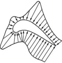
In gas turbine internal cooling application, the jet flow impinges on the target surface, ejecting a relatively cool turbulent air stream. Shear layer region, where the viscous forces affect the shear layer as the jet discharges, causing the jet to expand and develop. Wall jet region, where the jet flow impinges on the target surface, forms the wall jet and develops along the wall.
![Figure 9: Typical jet impingement structure before and after impingement [9]](https://thumb-ap.123doks.com/thumbv2/azpdfco/10576307.0/38.892.194.766.146.483/figure-9-typical-jet-impingement-structure-impingement-9.webp)
Literature Review
- Jet Impingement Cooling – Numerical Studies
- Jet Impingement Cooling-Experimental Studies
They found that the jet Reynolds number and the position of the jet nozzles significantly affect the heat transfer efficiency. They also observed that as the Reynolds number of the jet increased, the heat transfer at the surface also increased. Decreasing the jet-to-target distance and jet spacing improved heat transfer.
Numerical Formulation
- Governing Equations
- Continuity Equation
- Momentum Equation (Navier-Stokes Equations)
- Energy Equation
- Turbulence Modeling
- Turbulence Modeling Introduction
- SST k-ω Model
- Description of Physical Model
- Assumptions
- Meshing
- Mesh Description
- Wall Treatment Method
- Grid Independent Study
- CFD Solution
- Discretization Scheme
- Boundary Conditions
- Solver Setting
- Measure of Convergence
A combination of the Wilcox k– ω turbulence model and the k–ε model, known as the SST k– ω model, is adopted for the simulation. Menter [55] created the SST k-ω model to combine the precise and robust definition of the k-ω technique in the near-wall region with the free-stream independence of the k-ε model in the far field. The definition of turbulent viscosity is improved to simulate turbulent shear stress transport.
The k-ω-based SST model calculates the transport of the turbulent shear stress and provides unusually accurate predictions of the onset and amount of flow separation under an adverse pressure gradient. In the SST k–ꞷ model, the eddy viscosity does not remain constant to find the transport of the turbulent shear stress. This section describes the geometry and dimensions of the leading edge used to create the physical geometry under investigation.
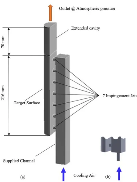
Significantly, the inlet supply channel and outlet sections of the semi-circular cavity are elongated (extended) to ensure uniform flow into and out of the geometry. A uniformly regulated cooling air cooling enters from the bottom of the supply channel, supplies the seven circular jets, enters the semicircular cavity, hits the target surface and discharges from the top to the bottom as the cavity is blocked from the bottom. The distance from the center of the leading edge to the rotating x-axis is Rarm = 50 cm.
The choice of solver settings in FLUENT is based on existing literature and guidelines of the near-wall 3D turbulence model.
Experimental Setup and Details
- Overview of Experimental Setup
- Test Facility
- Test Rig Description
- Compressed Air Supply
- Hot Gas Simulation
- Temperature Measurements
- Camera and Lighting Setup
- Test Section
- Experimental Procedure
- Validation Test Cases
The pressure inside the test section is regulated to the specific value by adding one more rotary union to the cooling air outlet. A homemade helical heat exchanger is designed to heat the cooling air to the required temperature. A digital flow meter measured the total flow rate moving to the feed channel for Rej = 7,500.
Since some losses occurred from the heat exchanger in the test section due to convection heat transfer, the inlet temperature is measured at the leading edge inlet. In general, the heat flux is not uniformly distributed over the leading edge surface in the actual turbine blade due to the root and tip flow behavior of the blade. Based on the actual gas turbine blade shown in Figure 21, the maximum temperature due to convection occurred almost at the center of the turbine blade, but in this experiment and CFD simulation, the researchers assumed a uniform heat flux along the target surface.
An adapter is attached to the bottom of the leading edge that connects to the hose, preventing leakage. The temperature of the cooling air going to the test section is controlled by a heat exchanger located between the tanks and the test section. Cooling air temperature is monitored at three locations: one thermometer at the compressor outlet and swivel inlet, and the primary thermometer using a T-type thermocouple at the leading edge inlet.
After controlling the coolant mass flow rate and its temperature to the test section, a 19-20V DC power supply drives the leading flexible heater.

Results and Discussion
Validation
- Temperature Contours Evaluation
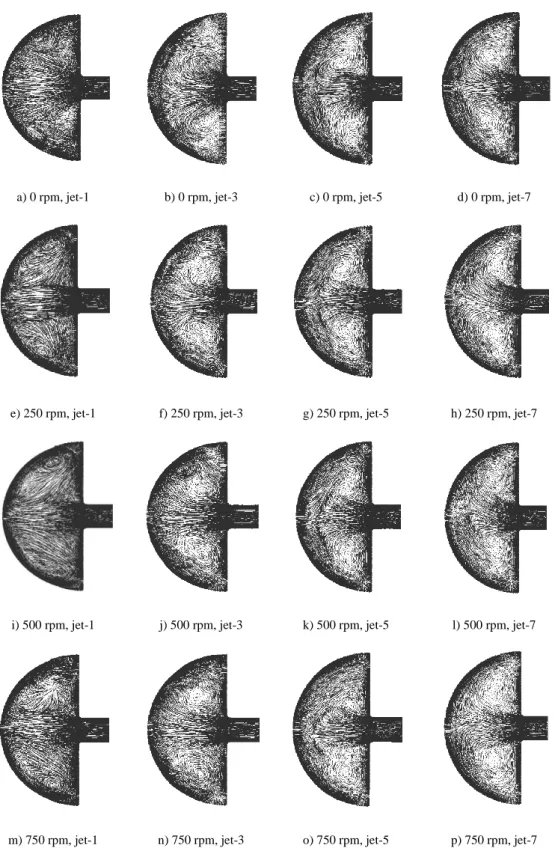
- Impingement Flow Behavior
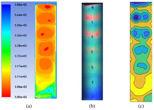
The thickness of the leading edge is zero thickness in the numerical analysis and 4 mm in the actual experiment. The second dataset used for validation is presented in Figures 32 to 36, consisting of the localized temperature of the surface thermocouple at the centerline of the leading edge corresponding to the seven locations of the jet; and two distributed leading-edge centerline temperatures obtained from numerical analysis and TLC-calibrated temperature contours. The unexpected behavior of jets one and two is also adequately covered in the experiment and numerical analysis.
As shown in Figure 27, the jet impingement region for jet aircraft had one and two higher temperatures than the other jet impingement regions. As shown in Figure 32 to Figure 36, the temperature values for beams three, four and five under all rotation speeds were in excellent agreement (±1%). The CFD results for jets one and two overestimate the thermocouple readings and the TLC calibrated temperature measurements as well.
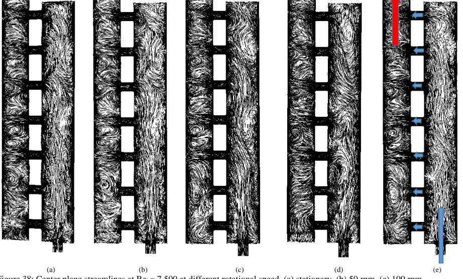
Comparing the results for jets one and two in Figure 32 to Figure 36 means that as the rotation speed increases, the deviation between the numerical results and the experimental data also increases. Two additional figures from the numerical analysis have been generated and presented to explain the temperature distribution contour, as shown in Figure 37 and Figure 38. The CFD results for jets one and two overestimated the experimental temperature because the CFD model did not account for lateral heat transfer in the thickness of the acrylic material.
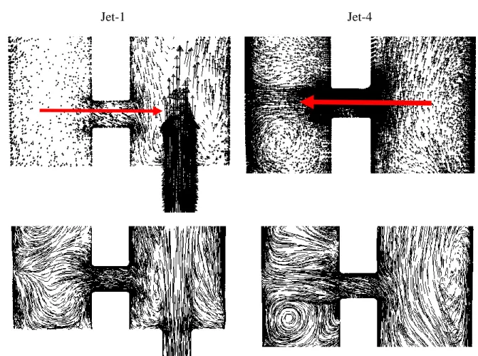
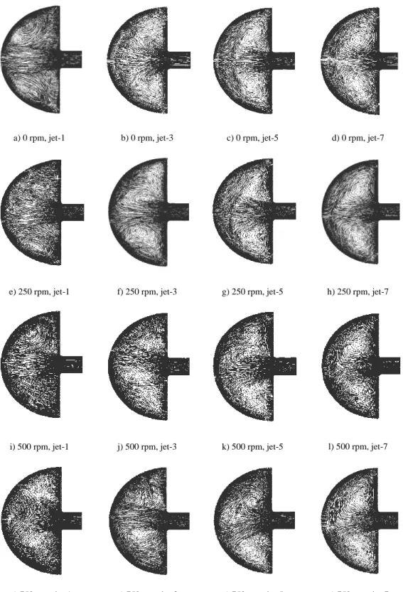
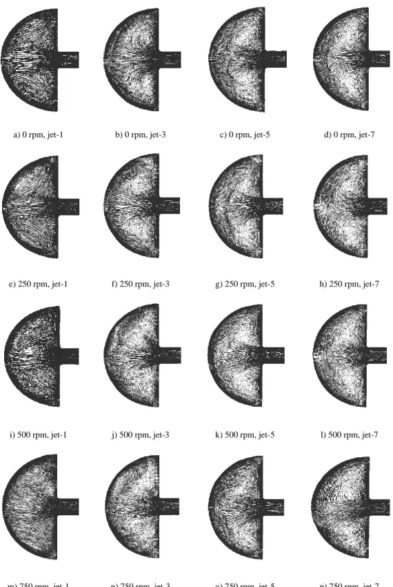
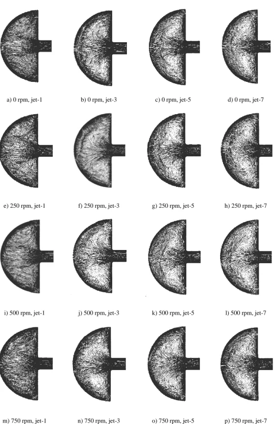
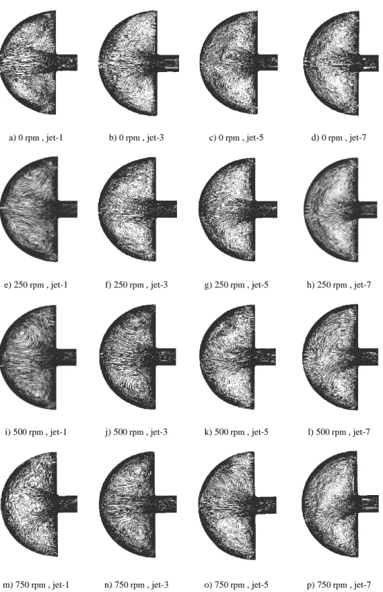
A careful examination of the streamlines for the central cross-sectional area is shown in Figure 38.
Numerical Results for the Modified Test Section
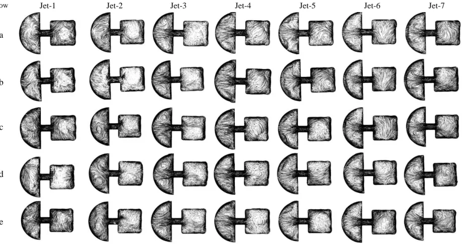
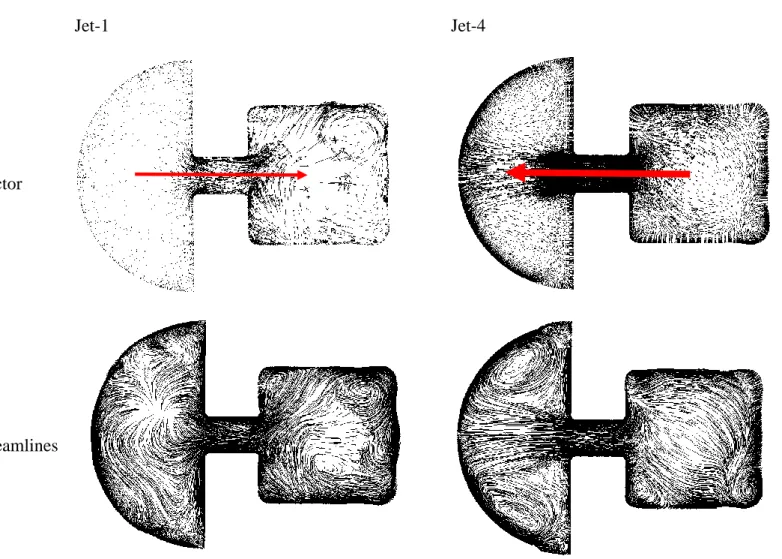
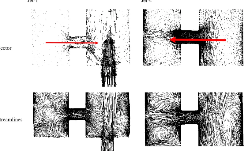
- Streamlines of Cross-Sectional Area for Each Jet
- Center Plane Streamlines
- Nusselt Number Contour
- Nusselt Number Distribution on Facing Each Jet
- Static Pressure Distribution Facing Each Jet
- Static Pressure Variation on the Center Line
- Nusselt Number Distribution on the Line
- Averaged Local Nusselt Number Facing Each Jet
- Mass Fraction for Each Individual Jet
- Pressure Coefficient for Each Individual Jet
- Correlation
The choice of the local Nusselt number shifted to the sides due to the deflected jet impingement caused by the rotation. The local Nusselt number for each jet has a minimum displacement at any rotation at a high Reynolds number. The localized Nusselt number on the semicircular curve line opposite each jet is plotted around the curved line in Figure 63 through Figure 68 for all Reynolds numbers of the jet aircraft.
At higher jet Reynolds numbers, such as Figure 68, the Nusselt number distribution from each jet shows less variation, exhibiting overall Nusselt number uniformity. For low jet Reynolds numbers, the Nusselt number distribution does not remain uniform, and the local Nusselt number for each jet is much higher than the average Nusselt number compared to higher Reynolds numbers. The minimum local Nusselt number occurred for jets one and two at low Reynolds number and high rpm.
As shown in Figure 76 (f), the angular velocity affects the local Nusselt number insignificantly at high Reynolds numbers, indicating that the jet inertial force is more important than the centrifugal force. In Figure 77, the average local Nusselt number on the curved surface facing each stream is shown. Mainly at low jet Reynolds numbers, the rotation speed significantly affects the local Nusselt number.
In general, the local Nusselt number for jets one to four is higher than jets five to seven. At low jet Reynolds numbers, Figure 77(a) and (b), the centrifugal force dominates, pushing the jet flow radially and weakening its Nusselt number. This environment reduced the jet collision for jets one and two, lowering the local Nusselt number for the first two jets, mainly at high rotation speed.
Conclusion and future work
Conclusions
The SST k- turbulence model with y+ of order 1 is a suitable model to simulate internal channel jet forcing under crossflow and rotating system. Both experimental measurements and numerical results, namely the temperature distribution along the centerline of the front target surface, show a very good agreement for nozzles number 3, 4 and 5. The results reveal the importance of the size of the inlet for the cooling air and its effect on the flow, which could eliminate jet shock from jets near the entry area.
A CFD analysis can overestimate or underestimate an experimental result, especially when the CFD model does not account for minor features of the problem, such as the wall thickness and inner step lip of the exhaust. The rotational speed causes a drop in total heat transfer, mainly at low jet Reynolds numbers, while it has an insignificant effect at high jet Reynolds numbers. In general, jet impingement is an efficient method of cooling the leading edge of the gas turbine blade.
Cooling performance at low jet Reynolds numbers is strongly influenced by individual jet location and rotation speed. Leading-edge rotation has a significant influence on the flow at low Reynolds numbers and has hardly any effect at high Reynolds numbers.
Future work
Song, Numerical study on flow and heat transfer characteristics of vortex cooling on leading edge model of gas turbine blade. Metzger, Local heat transfer in internally cooled turbine airfoil leading edge regions: Part I—Impingement cooling without film coolant extraction. Lin, G., et al., Numerical investigation on heat transfer in an advanced new leading edge impingement cooling configuration.
Liu, L., et al., The effect of tangential jet impingement on blade impact edge heat transfer. Zhou, T., et al., Numerical analysis of heat transfer by turbulent round jet at high temperature difference. Rao, Numerical investigations of heat transfer and pressure drop characteristics in a multi-jet system.
Metzger, D.E., et al., Heat transfer characteristics for inline and staggered arrays of cross-flow exhaust circular jets. Deng, H., et al., Experiments on shock heat transfer by film extraction flow at the leading edge of rotating blades. Elston, Experimental investigation of heat transfer in a leading edge, two-pass serpentine transition at high speeds.
Alvin, Effects of rotation on heat transfer for a single row jet impingement array with cross flow.