Correctly performing such tests requires a deep knowledge of how to treat the estimating equations of the parameters of the candidate distribution from a censored sample. The corresponding critical value of the test must be changed according to the type of. Yet they predetermined the timing of the test and built their estimates based only on the observed errors.
This is because AD gives more weight to the tail, whereas CVM gives more weight to the middle of. Therefore, together it will give a satisfactory picture of how close the theoretical and empirical distributions are. Formulas (2) and (3) are the test statistics for complete samples of life when all the tested items have failed before the end of the test.
A convenient and simple explanation of the mathematical details of this type of censoring can be found in [10]. The area under the probability distribution of the test statistic to the right of the critical value is called the significance level of the test. On the other hand, the area to the right of the data test statistic is called the p-value of the test.
For the log-normal distribution, the estimation equations (16) and (17) of the MLEs 𝜃̂𝑐𝑒𝑛 and 𝜏̂𝑐𝑒𝑛 from censored samples are both non-improvable implicit functions of 𝜃̂𝑐𝑒𝑛 and 𝜏̂𝑐𝑒 𝑛.
The pseudo code of the goodness-of-fit algorithms
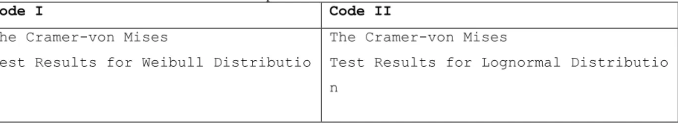
The pseudocodes of CVM and AD test are very similar, and differ only in the formula of the test statistics, namely in steps 3) and 4) in the following bullet points that describe the pseudocodes of both tests. The Mathematica codes of Cramér–von Mises and Anderson–Darling tests for Weibull and lognormal distributions.
The Mathematica codes of Cramér–von Mises and Anderson-Darling tests for Weibull and lognormal distributions
12 Mathematica and will automatically be colored light blue or gray when typed in the program depending on the Mathematica version used. Like MATLAB, semicolons (;) are placed at the end of some commands to print their output, and some other commands do not have semicolons because we need to see their output. As is clear from the first point in the pseudo code, users must enter the data of the censored dataset) to be tested. Full sample size (n), a positive integer that is equal to the number of values in the full sample, where the full sample consists of observed (data) failures and unobserved failures due to censoring.
Number of simulated samples (M), a large positive integer equal to the number of runs or loops used to generate the large set of test statistics. The first part of the codes is marked with (*[1]*) and consists of five entries highlighted in red that inform the user to enter these quantities. 13 codes calculate the MLE parameters by solving the estimation equations (10) and (11) for the Weibull or (16) and (17) for the log-normal presented in Section 1 .
The estimating equations are solved using the built-in function "FindRoot", which searches for a solution using the Newton–Raphson method and requires initial estimates of the parameters. The most important part of the code is (*[4]*), in which the code simulates a large number of random test statistics generated by Monte Carlo simulation. The idea is very simple because we only need to generate a large number of random censored samples and then calculate their corresponding test statistics.
The CV is usually chosen as the 0.95th percentile corresponding to the significance level (sl) of 0.05 which is already partially inserted (*[1]*). Then the simulated PV is the percentage of the simulated test statistics that are more than TS. The reader may notice that the built-in function "Quiet" is partially (*[5]*) used to silence Mathematica to avoid showing the messages about the accuracy of the calculations of some generated samples.
Also, the generated test statistic values are provided with the function Re[] inside the critical value command to consider only the real parts of some generated test statistic with non-zero imaginary part. This command excludes any indeterminate value of the test statistics that may occur due to many reasons such as the simulated censored sample size is 0 or an error that may occur while solving the MLE estimation equations. In the last part (*[6]*) we only show the quantities we need to see, these are the estimated parameters that are partly calculated (*[2]*), and the CV and PV that are partly determined (* [ 5]*), in addition to the decision of the test as “accept” if PV>sl or “reject” otherwise.
The Cramér–von Mises test Mathematica code for Weibull distribution
The Cramér–von Mises test Mathematica code for the lognormal distribution
The Anderson-Darling test Mathematica code for Weibull distribution
The Anderson-Darling test Mathematica code for the lognormal distribution
Illustrative Examples
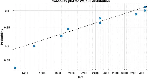
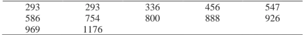
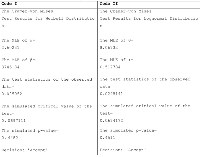
At the lower temperature intensity T3, the test took a long time to cause failures and the experiment was stopped after the 9th cell failure. Cell failure times are not explicitly reported in [1], where the authors present them through Weibull probability plots to graphically demonstrate the fit of the data to this distribution. Now let us test the fit of the data to the two models considered in this work using the CVM and AD test codes for the censored data presented in Section 3.
For example, the MATLAB CVM (cmtest) function for the Weibull distribution requires the input of estimates of its parameters, the measure β, and the shape parameters α. PV, TS, and CV are the p-value, test statistic, and critical value of the test, respectively. The data points fall on or near the straight line of the Weibull distribution, indicating its goodness of fit to the data [21].
On the other hand, if one tries to find the maximum likelihood estimates for the given data using the built-in command "wblfit" of MATLAB, the result will be β=2716.8 and α=3.4000, which are different but comparable with the correct estimates mentioned above, β=3745.84 and α=2.60231. This wide difference between the two decisions demonstrates the shortcomings of the command and the error that practitioners would make. The same incorrect result can be seen on Mathematica when using the built-in command CramerVonMisesTest[data, WeibullDistribution produces a p-value of 0.0444 declaring the rejection of the Weibull distribution and this is completely wrong.
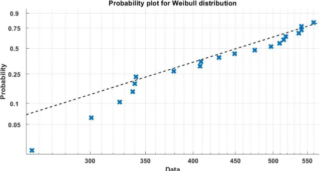
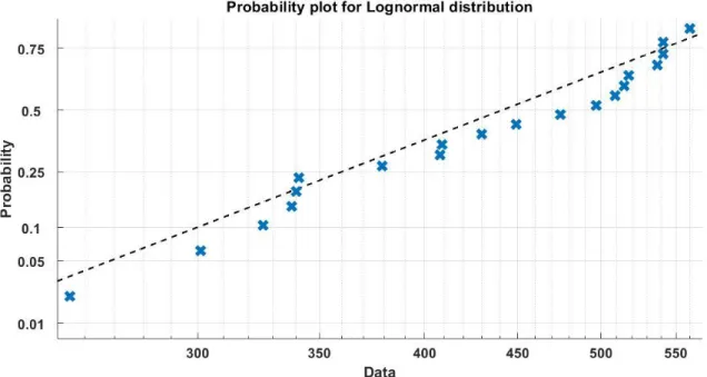
The plot of the lognormal distribution is very similar to that of the Weibull, but the former has a clearly better fit on the left tail of the data. It is clear from the two plots that Weibull and lognormal fit the observed data correctly. We can notice from the two figures that the lognormal distribution captures more points on its left tail, whereas the Weibull better controls the center of the data.
The US Department of Energy estimates that solid-state lighting fixtures are expected to save $250 billion in energy costs over the next 20 years and avoid 1,800 million metric tons of CO2 [24]. Reliability remains one of the challenges, hindering further diffusion of this technology, and there is a crucial need for the lighting industry and research centers to understand the durability and failure models of the solid state lighting. In this example, we will apply the two codes in testing the compliance of the sensored solid state lighting (SSL) fixture experimental data from the hammer test of [24].
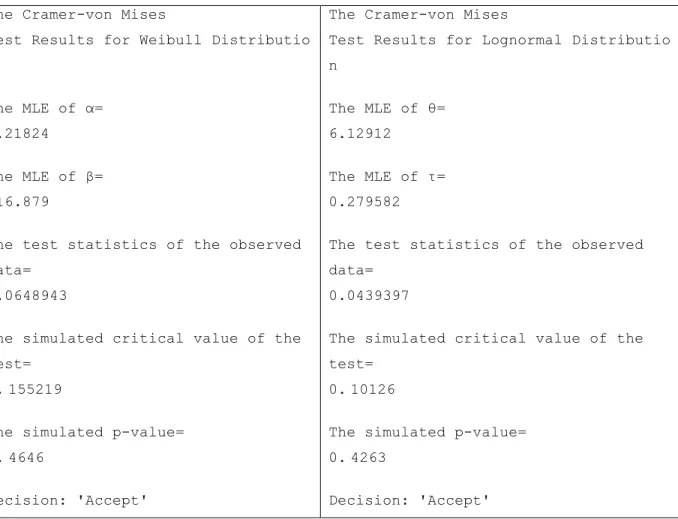
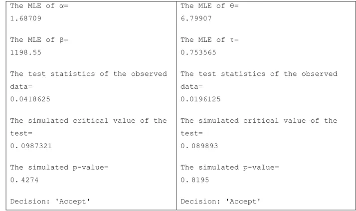
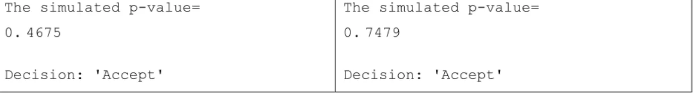
Like Examples 4.1 and 4.2, the following are the inputs and outputs of the two tests. These results agree with the probability plots of the two distributions as illustrated in Figures 5 and 6, and with the conclusion of [10].
Conclusions and suggestions
Using a normal speed computer, for Weibull distribution, both CVM and AD codes need about 0.5 minute, when the number of simulations is 5000 for size 10 samples, up to 5 minutes, for 20000 sample size simulations 30, while for the log-normal distribution, the codes last less than these times. 1] Espinet-González P, Algora C, Núñez N, Orlando V, Vázquez M, Bautista J, and Araki K (2014) Temperature-accelerated lifetime test on commercial concentrator III-V triple-junction solar cells and reliability analysis as a function of operating temperature. 10] Kittaneh OA, Majid MA (2019) Comparison of two lifetime models of solid-state lighting based on sup-entropy.
11] Kittaneh OA, Helal S, Almorad H, Bayoud HA, Abufoudeh G, Majid MA (2021) Preferred parametric model for the lifetime of the organic light-emitting diode under accelerated current stress tests.