Examples are also provided to illustrate the use of these techniques in risk management. The most advanced and exotic simulation topics in financial engineering and risk management are presented here.
QUESTIONS
SIMULATION
Through simulations, one learns about the different characteristics of the model, the behavior of the phenomenon and features of the approximate solutions. It helps us visualize the model, study the model and improve the model.
EXAMPLES
Quadrature
This rule approximates the integral by the sum of the areas of rectangles with base ( b - U)/. We will not go into details here, but interested readers may refer to Conte and de Boor (1980).
Monte Carlo
First, we might want to calculate the expected value of a random variable X with probability distribution function (p.d.f.) f ( x. In addition to the Monte Carlo method, we should also mention that the idea of the quasi-Monte Carlo method has also received much attention on the most recent.
These texts mainly discuss traditional simulation techniques without much emphasis on finance and risk management. The survey article by Broadie and Glasserman (1998) provides a concise description of the essence of simulations in finance.
EXERCISES
INTRODUCTION
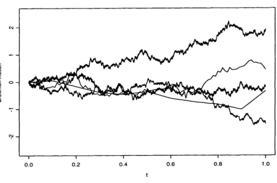
WIENER’S AND IT6)’S PROCESSES Consider the model defined by
The idea is that by taking the limit as n tends to cm, the process S[] will tend to a Wiener process in distribution. In this case, the solution X (t) can be analytically written down in terms of the parameters p and (T) and the Wiener process W (t.
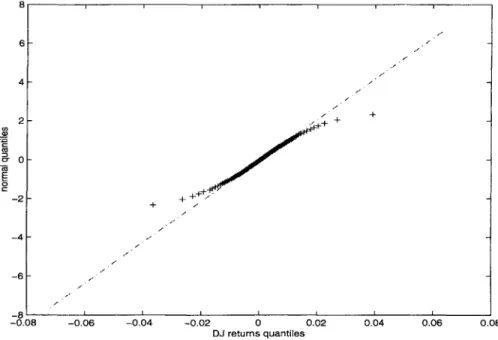
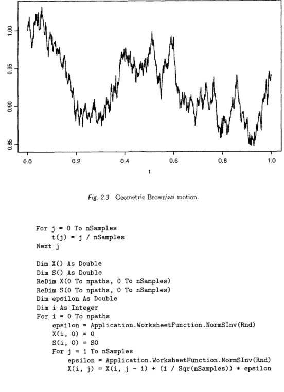
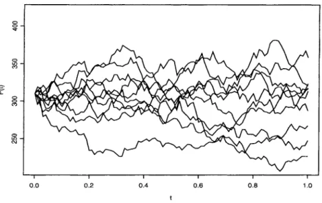
STOCK PRICE
The geometric Brownian motion S ( t ) drifts closer to zero as time goes on, but its mean value E(S(t)) is constantly increasing. This example demonstrates the fact that the average function can sometimes be misleading in describing the process.
The first two terms of the above expression are of higher order than At, so we can omit them, since we only want terms up to the order of A t. If we multiply the integrative factor ePt on both sides of the SDE, we get e-t dXt = ePtXt dt + e-t dWt.
EXERCISES
By integrating both sides of this equation. Then using the same method by considering the process U, = eptXt, it can be easily shown that the solution to this SDE is given by the process. One such process is known as the Ornstein-Uhlenbeck process, which is often used in bond price modeling. where XO = 0 and Wt is a standard Brownian motion process. a) Find the stochastic differential equation applicable to St. 10 and plot it on the same graph.
A stock price is governed by
INTRODUCTION
Note that the long position in a put option is different from the short position in a call option. A long position in an option always has a non-negative payoff, while a short position in an option always has a non-positive payoff, but the option premium is charged upfront.
ONE PERIOD BINOMIAL MODEL
THE BLACK-SCHOLES-MERTON Equation 35 This portfolio is risk-free if A is chosen such that the value of the portfolio remains the same for both alternatives, i.e. If the value of the option is today denoted by f, then the present value of the portfolio equal to.
THE BLACK-SCHOLES-MERTON EQUATION
Due to the no-arbitrage consideration, this risk-free profit should yield the risk-free rate. While these two examples are illustrated with a call option, similarly the same principle can be used to price a put option. Details can also be found in Hull (2006).
Theorem 3.1 Using the notation just defined, and assuming that the price and the bond are described by the geometric Brownian motion (3.1) and the
BLACK-SCHOLES FORMULA
EXERCISES
There is a call option on the stock that can only be exercised at the end of six months with an exercise price of $65. a). To establish a fully hedged position, what would (b) for each of the two options, what will be the value of your (c) what is the expected value of the option price at the end of the period.
A fixed strike geometric Asian call option has the payoff function max(GT- K,O) where
- INTRODUCTION
- RANDOM NUMBERS
- DISCRETE RANDOM VARIABLES
- ACCEPTANCE-REJECTION M E T H O D
Use the result of question 5. where CBS is the Black-Scholes formula for a call option with constant parameters. One of the most popular devices for generating uniform random numbers is the congruence generator.
Theorem 4.1 The acceptance-rejection algorithm generates a random vari- able X such that
- CONTINUOUS RANDOM VARIABLES
- The Rejection Method
- Multivariate Normal
- EXERCISES
- INTRODUCTION
- SCENARIO ANALYSIS
- Value at Risk
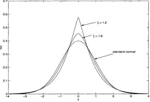
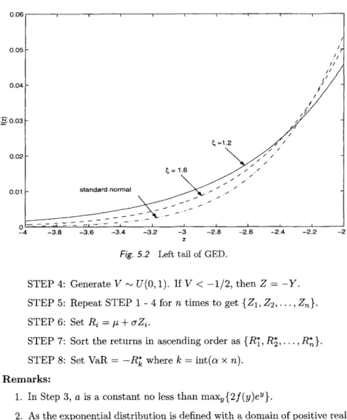
- Heavy-Tailed Distribution
- STANDARD M O N T E CARLO
- Simulating Option Prices
- Simulating Option Delta
- EXERCISES
- APPENDIX
- INTRODUCTION
- ANTITHETIC VARIABLES
- STRATIFIED SAMPLING
- CONTROL VARIATES
- IMPORTANCE SAMPLING
The SPLUS code of the likelihood function and the plot is given after this paragraph. The other one is the standard error CT of the output X, which can be improved by some techniques. 6.1, the vertical axis is the payoff and the horizontal axis is the value of z , the input standard normal.
Similarly, the variance of the estimate of the control variation is given by i 2 / n, where e2 is the regression estimate of 02. Recall the note that M (t ) = E(etx) represents the moment generating function (m.g.f.) of the variable random X with density f.
EXERCISES
INTRODUCTION
BARRIER OPTION
A down-and-in barrier call option is a cheaper tool to hedge the upside risk. From the definition, it can be easily seen that holding both a down-and-in and down-and-out options with the same strike price K and maturity T is the same as holding a "vanilla" option. Let c d c and c d o be the setting value for the down-and-in call and the down-and-out call, respectively.
LOOKBACK OPTION
There are lookback put-call parities that link the floating strike lookback call (put) with the fixed strike lookback put (call). It is interesting to note that simulating fixed strike lookback options requires less storage than simulating the floating ones. With this observation and the lookback-put-call parities, a stock-saving approach to simulating floating strike lookback options can be developed.
ASIAN OPTION
The reason is that the payouts of fixed lookback options do not depend on the final price of the ST asset. To value a call with a floating callback, a fixed callback price is simulated with a strike price equal to the realized minimum asset value. Using the analytical solution of the geometric Asian call, we simulate the arithmetic Asian price via the control variable.
AMERICAN OPTION
- Simulation: Least Squares Approach
- American-Style Path-Dependent Options
The coefficients of the polynomials are estimated from the data in Table 7.2 using the least squares method. In the regression equation (7.9), only in-the-money paths are used in the estimation of least squares because these paths are sensitive to immediate exercise. Keep in mind that the option holder will only exercise the option if it is in-the-money.
GREEK LETTERS
We illustrate these ideas with a down and out call option in the following example. Estimate the delta of a call option down and out with a strike price of 95 and a downside barrier reserve of 80. For example, gamma is the second-order partial differentiation of the option pricing formula relative to the asset's underlying price.
EXERCISES
American call option is never optimal to exercise before expiry if the underlying asset does not pay dividends. Modifying Example 7.4, simulate the price of an American call option with a strike of $12 and a yield of 6 of 4%. Based on financial acumen, a risk analyst speculates that the forward start call option is the discounted default call price.
INTRODUCTION
Complex multi-asset options, or structured products, may even include path-dependent features.
SIMULATING EUROPEAN MULTI-ASSET OPTIONS
CASE STUDY: ON ESTIMATING BASKET OPTIONS
On the other hand, we can use MC simulation to estimate the option price by assuming that individual asset follows the Black-Scholes dynamics. The option price is then evaluated by discounting the sample mean of the option payoff using the interest rate of 5%. We are also interested in the contribution of the error in the estimation of parameters of the option.
DIMENSIONAL REDUCTION
From (8.4) we see that the contribution of the term &viz, to the value of X decreases with the index i. When the sum of the first three eigenvalues is divided by the total, the ratio is close to 95%. By It6's lemma, we know that the final value of the ith asset is given by.
EXERCISES
Using the no-arbitrage argument, one deduces that the exchange option has the properties: Run the simulation program for the price exchange option and compare the numerical result with the analytical result. The so-called geometric basket option has the payout feature. a) Show that this option has a lower value than the usual basket option.
INTRODUCTION
DISCOUNT FACTOR
Note that the continuously compounded interest rate r and the annual interest rate R are connected by the formula. STOCHASTIC INTEREST RATE MODELS AND THEIR SIMULATIONS 161 evolution of discount factor B(t, T ) , which can be seen as the zero price at t with unit payment at T. The rate of return of this zero coupon effect must be the instantaneous interest rate ~ (t.
Since y(t, T ) is also defined as the return on a bond, the discrete return to maturity yt is given by. T } be the j-th rate path out of M sample paths generated by the previous algorithm with At. This closed formula allows us to check the accuracy of simulating the Vasicek model.
In practice, it is sometimes more important to know a bond's yield than its value because market experts are used to derive the bond's price from the yield curve. The first function can be solved by calculating the discount factor using the aforementioned method. For the second characteristic, we consider the Black-Scholes dynamics of funds in the framework of interest rate economics of the Villages.
EXERCISES
INTRODUCTION
BAYESIAN INFERENCE
Given a likelihood function, the conjugate prior distribution is a prior distribution such that the posterior distribution belongs to the same distribution class as the prior. Conjugate priors facilitate statistical inference because the posterior distributions belong to the same family as the prior distributions, which are usually of known shapes. In the one-dimensional case, deriving the conjugate priors is relatively simple when the likelihood belongs to the exponential family.
SIMULATING POSTERIORS
MARKOV CHAIN MONTE CARLO
- Gibbs Sampling
Gibbs sampling takes advantage of this fact and provides a way to reduce a multidimensional problem to an iteration of low-dimensional problems. Define pi and 0; be random variables generated in the ith iteration of the Gibbs sampling procedure. With all components ready, Gibbs sampling begins by choosing initial values of PO, a:, ko, XO, and sg.
METROPOLIS-HASTINGS ALGORITHM
In other words, a Markov chain whose limiting distribution is the posterior distribution can be constructed by finding a time-reversible Markov chain. We begin this process by specifying transition probabilities qij. qij has already satisfied the time reversibility, then the corresponding Markov chain is the one we want. Since we do not want to reduce the probability of moving from j to i, we set
EXERCISES
X , are independent observations that follow N(p, 0 2 ), where p is a known quantity. a) Show that the probability function L(02) satisfies. Show that if the probability function comes from the exponential family and the prior distribution is from the exponential family, then the posterior distribution also belongs to the exponential family. Compare your number with the GED-VaR defined in Chapter 5. n is a Poisson variable of mean A. Consider the normal distribution with an unknown mean p and a known variance. a) Suppose that the prior of p is a discrete mixture of two normal (b) Suppose that the prior of p is a discrete mixture of k normal den-.
CHAPTER 2
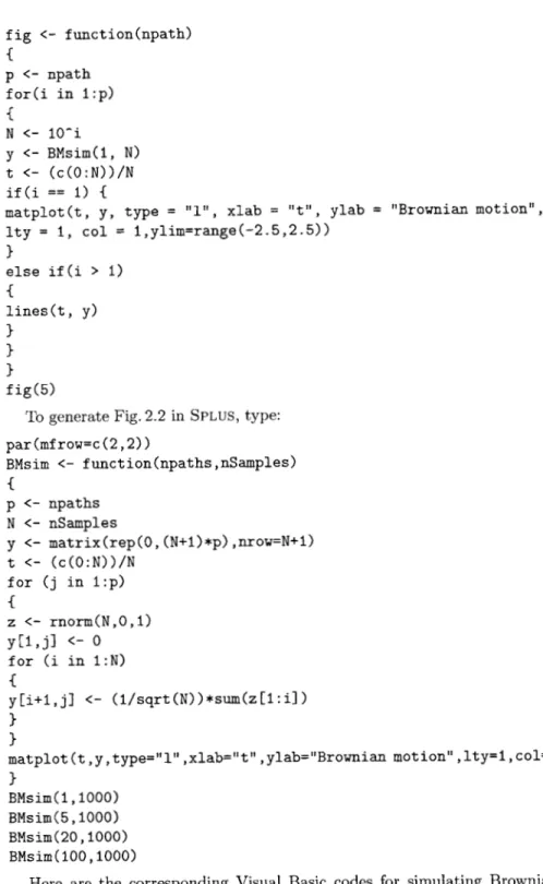
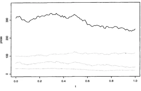
![Fig. 2.2 Sample paths of Brownian motions on [O,l].](https://thumb-ap.123doks.com/thumbv2/azpdfco/10578982.0/30.648.33.600.134.495/fig-2-2-sample-paths-brownian-motions-o.webp)