The DCAs are constructed based on the DC programming theory and the duality theory of J. Ordin and Bagirov, and by Bagirov based on the DCA in DC programming and the qualitative properties of the MSSC problem.
Basic Definitions and Some Properties
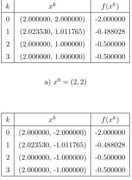
Fermat's rule for convex optimization problems states that ¯x ∈ Rn is a solution to the minimization problem. The next example, which is similar to example 1.1 in [93], shows that a fixed point need not be a local solution.
DCA Schemes
If we delete some real constants from the expression of the objective function (Dk), we get the following equivalent problem. 1.4) The objective function (Pk) is a convex upper approximation of the objective function (P). If we delete some real constants from the expression of the objective function (Pk), we get the following equivalent problem.
General Convergence Theorem
Note that the limit point xe of the sequence {xk} is the unique critical point of (P), which is neither a local minimizer nor a stationary point of (P). Since the construction of the sequences {xk} and {yk} does not depend on the choice of the constants ρ1, ρ∗1, ρ2 and ρ∗2, we have by assertion (i) of Theorem 1.1 for each k ∈ N the inequality.
Convergence Rates
To see this, it is sufficient to choose a constant β ∈ (0,1) that satisfies the condition stated in Definition 1.9, put µk = βkxk−1 −xk¯ for all k ≥ 1, and note that kxk−xk ≤¯ µk for all k large enough, while {µk} converges Q-linearly to 0 because µk+1 ≤ µk for all k is large enough. Then there is a sequence of nonnegative scalars {µk} such that kxk −xk ≤¯ µk is large enough for all k, and {µk} converges Q-linearly to 0.
Conclusions
Analysis of an Algorithm in Indefinite Quadratic
Convergence and Convergence Rate of the Algorithm
Equivalently, xk+1 is the unique solution of the highly monotonic affine variation inequality given by the affine operator x 7→ (Q + ρE)x + q − ρxk and the polyhedral convex set C. 2.12) The convergence and the convergence speed of algorithm B, the proximal DC decomposition algorithm, can be formulated as follows. Therefore, the computational error between the obtained approximate solution xk and the exact limit point ¯x of the sequence {xk} is less than the number Ck.
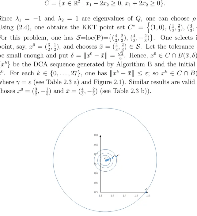
Asymptotical Stability of the Algorithm
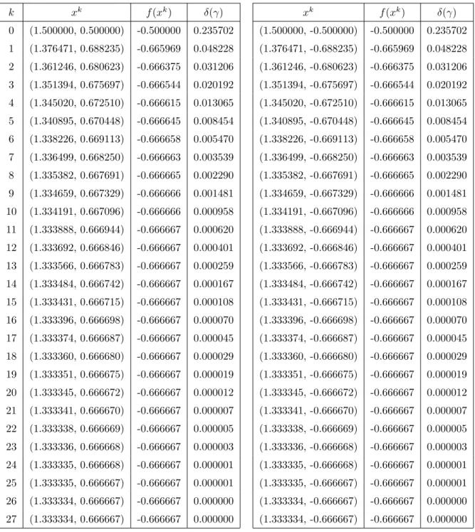
In other words, x¯ is asymptotically stable with respect to 2.27) First, we show that the statement about the stability of DCA sequences generated by algorithm B is valid for a chosen number δ > 0. Then, to obtain the statement about the attractiveness of DCA sequences generated by generates algorithm B, we observe with the stability result just obtained that for any γ > 0 there exists δ = δ(γ) > 0 such that if x0 ∈ C ∩ B(¯x, δ) and if {xk} is a sequence DCA generated by algorithm B and the starting point x0, then property in (a) holds. Moreover, for each j there exists some x0,j ∈ C ∩ B(¯x, δj) such that the DCA sequence {xk,j} generated by algorithm B and the starting point x0,j does not converge to ¯x.
Without loss of generality, we can assume that the entire sequence {xej} is contained in Fα.
Influence of the Decomposition Parameter
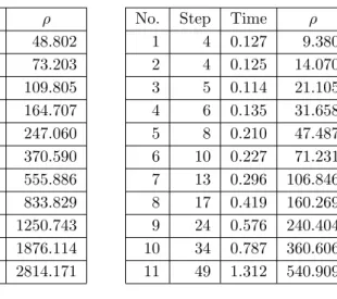
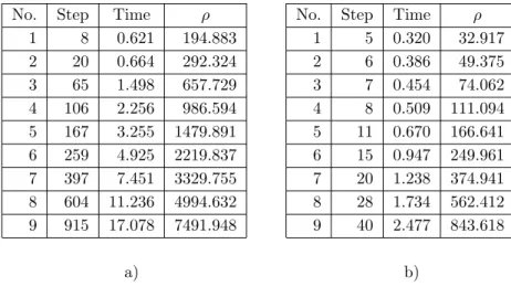
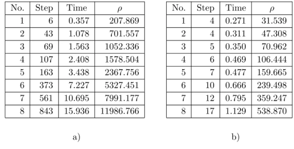
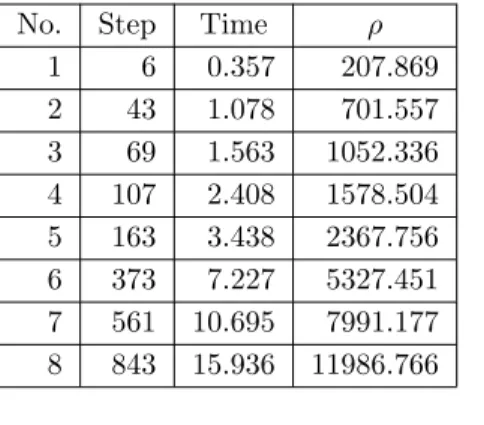
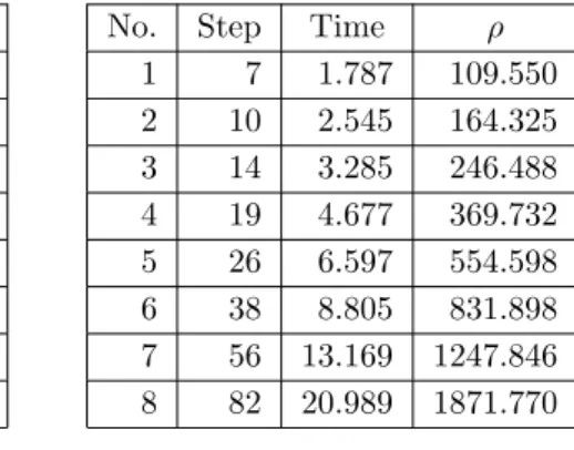
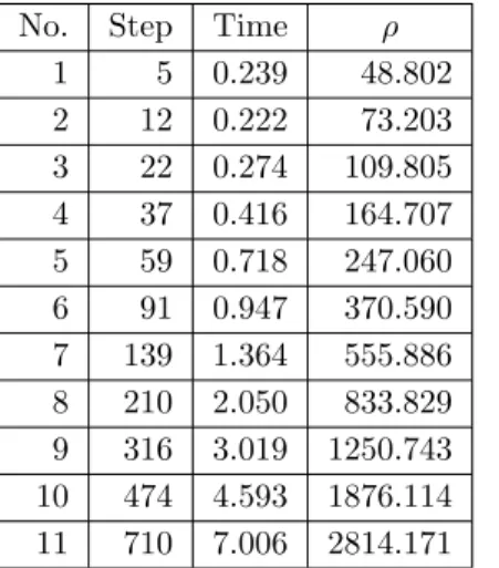
In Table 2.4, the second row in sub-tables a) and b) corresponds to the minimum decomposition parameters for Algorithm A and Algorithm B, respectively. The decomposition parameters for the test reported in the third row are 1.5 times the minimum decomposition parameters. The decomposition parameters for the test reported in the fourth row are 1.5 times the decomposition parameters just mentioned; and so on.
In sub-tables a) and b), the first column indicates the serial number of the tests. For any row of subtables a) and b) with the same sequence number, the number of steps required by algorithm B is much less than that required by algorithm A. • For any row of subtables a) and b) with the same sequence number the running time of Algorithm B is much shorter than Algorithm A. Thus, in terms of the number of computational steps and execution time, Algorithm B is much more efficient than Algorithm A when the algorithms were applied to the same problem.
Conclusions
Qualitative Properties of the Minimum Sum-of-Squares
Basic Properties of the MSSC Problem
A component ¯xj of ¯x is said to be attractive with respect to a data set A if the set is. Ak} is a natural clustering associated with the global solution x¯ from (3.2), then Aj is nonempty for every j ∈ J. Thus, there is no loss of generality in the assumption that a1, .., am are pairwise distinct points.
Since the minimum of finitely many continuous functions is a continuous function, the objective function of (3.2) is continuous on Rnk. If at least one index j ∈ J exists with kxj−a0k > 2ρ, denote the set of such indices by J1 and define a vector. Since there are only finitely many nonempty subsets Ω ⊂ I, the set B of vectors bΩ is defined by formula bΩ = 1.
The k-means Algorithm
To understand the significance of the above results and those to be determined in the next two sections, let us recall the k-means clustering algorithm and consider an illustrative example. After the clusters are formed, for each j ∈ J, if Aj 6= ∅ then the center xj is updated by the rule. Based on existing knowledge on the MSSC problem and the k-means clustering algorithm, it cannot be known whether the five centroid systems obtained in points (a)-(e) of Example 3.1 contain a global optimal solution to the clustering problem. , or not.
Even if we know that the centroid systems obtained in (a) and (c) are the global optimal solution, we still cannot say for sure whether the centroid systems obtained in (b), (d), (e), local optimal solutions (3.2) or not. In particular, it will be shown that the centroid systems in (a) and (c) are global optimal solutions, the centroid systems in (b) and (d) are local-non-global optimal solutions, while the centroid system in (e) is not a local solution ( despite the fact that the centroid systems generated by the k-means algorithm converge to it and the value of the objective function is the same for it.
Characterizations of the Local Solutions
According to (3.17), the first statement of the following theorem means that if x is a nontrivial local solution, then for each data point ai ∈ A there exists a unique component xj of x such that ai ∈ A[xj]. Therefore, given the continuity of the functions hi,j(x), there exists an open neighborhood Ui of x such that. Therefore, combined with Theorem 3.3, the following statement gives a complete description of non-trivial local solutions of (3.2).
Thus ¯x is a local solution which does not belong to the global solution set, i.e. ¯x is a local-non-global solution of our problem. The algorithm can provide a global solution, a local-non-global solution, as well as a centroid system which is not a local solution. In other words, the quality of the obtained result depends to a large extent on the initial center of gravity system.
Stability Properties
The above analysis shows that the k-means algorithm is very sensitive to the choice of starting centroids. According to Theorem 3.1, problem (3.2) has solutions and the number of global solutions is finite, that is, F(¯a) is nonempty and finite. For each ω ∈ Ω, from the above observations we can deduce that the function gω(a) := f(xω(a), a) is locally Lipschitz on Rnm.
Thanks to Theorem 3.1, we know that the global solution set F(a) of (3.2) is in the set.
Conclusions
Some Incremental Algorithms for the Clustering Prob-
Ordin-Bagirov’s Clustering Algorithm
- Basic constructions
- Version 1 of Ordin-Bagirov’s algorithm
- Version 2 of Ordin-Bagirov’s algorithm
- The ε-neighborhoods technique
Next, we apply the k-means algorithm to problem (4.8) starting from the set Ω defined by (4.17) to find Ae4. In the above example, centroid systems resulting from both Algorithm 4.1 and Algorithm 4.2 belong to the global solution set of (3.2), which consists of the two centroid systems in (4.24). Algorithm 4.1 thus yields one of the four centroid systems in (4.25), which is a local, non-global solution of our clustering problem (see Remark 4.1 for detailed explanations).
Next, we apply the k-means algorithm to problem (4.8) with starting points from the set Ω defined by (4.17) to findAe4. Remarkable properties of Algorithm 4.2 are described in the following theorems, where the following assumption is used: Thus, the centroid system resulting from Algorithm 4.2 is a very good candidate to be a non-trivial local solution of (3.2).
Incremental DC Clustering Algorithms
- Bagirov’s DC Clustering Algorithm and Its Modification 81
- The Fourth DC Clustering Algorithm
From our experience of implementing Procedure 4.3, we know that the stopping criterion = ∇g(xp) slows down the computation too much. In step 4 of procedure 4.3 (respectively, step 3 of procedure 4.4), the convex differentiable program must be chosen. If the computation in Procedure 4.5 (respectively, in Procedure 4.6 with a tolerance ε = 0) does not terminate after many finite steps, then the iteration sequence {xp} converges to a stationary point of (4.35).
To prove this assertion, it suffices to construct a suitable example, where the computation from Procedure 4.5 does not terminate after many finite steps. However, the computation does not terminate at any step p, because the stopping criterion in Step 5 (which requires xp to be the barycenter of Ωp = A1(xp) ∪ A4(xp) = {a3}) is not satisfied. ii) To show that the computation from Procedure 4.6 with ε = 0 may not terminate after many finite steps, we consider the above two-dimensional clustering problem. If the computation by Procedure 4.8 with ε = 0 does not terminate after finitely many steps, then, for each j ∈ {1,. i).
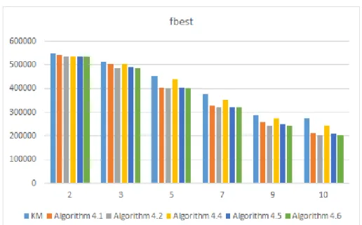
Numerical Tests
It is clear that, in terms of the best value of the cluster function, Algorithm 4.2 is preferable to Algorithm 4.1, Algorithm 4.5 is preferable to Algorithm 4.6, Algorithm 4.2 is preferable to KM, and Algorithm 4.5 is also preferable to KM. This is the reason why the incremental clustering algorithms just mentioned usually produce better values of the cluster function than KM.
Conclusions
Ravi, Clustering with constraints: Feasibility issues and the k-means algoritme, I: Proceedings of the 5th SIAM Data Mining Conference, 2005. Wang, Billedforbedring baseret på kvadratisk programmering, Proceedings of the 15th IEEE International Conference on Image Processing, s. Kasabov, Robust kernetilnærmelse til klassificering, Proceedings of the 24th International Conference “Neural Information Processing”, ICONIP 2017, Guangzhou, Kina, November Proceedings, Part I, pp.
MacQueen, Some methods for classification and analysis of multivariate observations, Proceedings of the 5th Berkeley Symposium on Mathematical Statistics and Probability, pp. Xia, A cutting algorithm for the minimum sum-of-squad error clustering, Proceedings of the SIAM International Data Mining Conference, 2005. Wang, Solving indefinite kernel support vector machine with difference of convex function programming, Proceedings of the Thirty-First AAAI Conference on Artificial Intelligence (AAAI-17), Association for the Advancement of Artificial Intelligence, pp.