ANY USE OF THE WORK EXCEPT AS AUTHORIZED IN THIS LICENSE OR COPYRIGHT LAW IS PROHIBITED. BY EXERCISING ANY RIGHTS TO THE WORK CONTAINED HEREIN, YOU ACKNOWLEDGE AND AGREE TO BE BOUND BY THE TERMS OF THIS LICENSE.
Main Ideas
The second idea of the book is that certain quantities are random, but even random numbers have patterns that we can capture using tools such as distributions and correlations. In the chapter on parallel algorithms, we learn how to distribute those iterations across multiple parallel processes, and how to split individual iterations into independent steps that can be executed simultaneously on parallel processes, to reduce the total time it takes to complete a solution within a specific goal. precision.
About Python
Book Structure
In the examples we look at complex algorithms such as Shannon-Fano compression, a maze solver, a clustering algorithm and a neural network. In the message passing case, we create a simple "parallel simulator" (psim) in Python that allows us to understand the basic ideas behind message passing and problems with different network topologies.
Book Software
In the GPU case, we use pyOpenCL[4] and ocl[5], a Python-to-OpenCL compiler that allows us to write Python code and convert it to OpenCL in real time for execution on the GPU.
Acknowledgments
About Python
- Python versus Java and C++ syntax
- help, dir
There are many interpreters and compilers that implement the Python language, including one in Java (Jython), one built on .Net (IronPython), and one built in Python itself. The Python language provides two commands to obtain documentation about objects defined in the current scope, whether the object is built-in or user-defined.
Types of variables
The exponent of the smaller number is increased to the exponent of the larger number. Different keys and values in the same dictionary need not be of the same type.
Python control flow statements
The parameters for range(a,b,c) are as follows: the first parameter is the initial value of the list. Function f creates new functions; note that the scope of the name g is completely cool internally.
Classes
- Special methods and operator overloading
- class Financial Transaction
MyClass() calls the class's constructor (in this case, the default constructor) and returns an object, an instance of the class. All variables are local variables of the method, except variables declared outside methods, which are called class variables, equivalent to C++ static member variables, which have the same value for all instances of the class.
File input/output
What is the net present value at the beginning of 2012 for a bond that pays $1,000 on the 20th of each month for the next 24 months (assuming a fixed interest rate of 5% per year).
How to import modules
We use the uuid4 function, which also uses the machine's time and IP address to generate the UUID. One of the best features of Python is that it can introspect itself, and this can be used to compile Python code just-in-time into other languages.
Order of growth of algorithms
- Best and worst running times
Often we cannot precisely determine the runtime function, but we may be able to set bounds on the runtime. To calculate the worst-case running time, we assume that the maximum number of calculations are performed. Under each of the two scenarios, we calculate the runtime by counting the number of times the most nested operation is executed.
Because there are no nested loops, the time to execute each iteration of the loop is almost the same, and the execution time is proportional to the number of iterations of the loop.
Recurrence relations
- Reducible recurrence relations
This means that the execution time of the join is proportional to the total number of values they can include from ptor. We transformed the problem of computing the running time of the algorithm into the problem of solving the recurrence relation. Other recurrence relations do not immediately fit one of the previous patterns, but often they can be reduced (transformed) to fit.
Note that there are recurrence relations that cannot be solved by any of the methods described.
Types of algorithms
- Memoization
We can refactor the merge sort algorithm to eliminate repetition in the algorithm implementation, while keeping the logic of the algorithm unchanged. When the algorithm terminates, we hope that the local optimum is equal to the global optimum. If this is the case, then the algorithm is correct; otherwise, the algorithm produced a suboptimal solution.
Memoization consists of allowing users to write algorithms using a naive divide-and-contrast approach, but functions that may be called more than once are modified so that their output is cached are called, and if they are called again with the same initial state, instead of the algorithm running again, the output is fetched from the cache and returned without any calculations.
Timing algorithms
Data structures
- Arrays
- List
- Stack
- Queue
- Sorting
A queue data structure is similar to a stack, but while the stack returns the most recently added item, a queue returns the oldest item in the list. Any addition or deletion of an element at the beginning of a list requires all elements in the list to be shifted by one. In fact, this algorithm is linear in the range of the elements of the input array.
Note that here we also calculated Tmemory, for example the order of growth of memory (not of time) as a function of the input size.
Tree algorithms
- Heapsort and priority queues
- Binary search trees
- Other types of trees
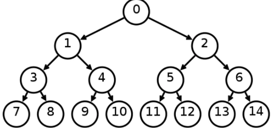
We can also count the nodes from top to bottom and from left to right, as in the image. A heap can be used to implement a priority queue, for example, storage from which we can efficiently retrieve the largest element. This means we can search by simply traversing the tree from top to bottom along a path down the tree.
This can be generalized to trees for which each node has children and stores more than one value.
Graph algorithms
- Breadth-first search
- Depth-first search
- Disjoint sets
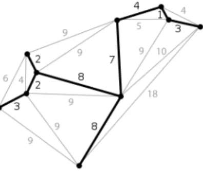
- Minimum spanning tree: Kruskal
- Minimum spanning tree: Prim
- Single-source shortest paths: Dijkstra
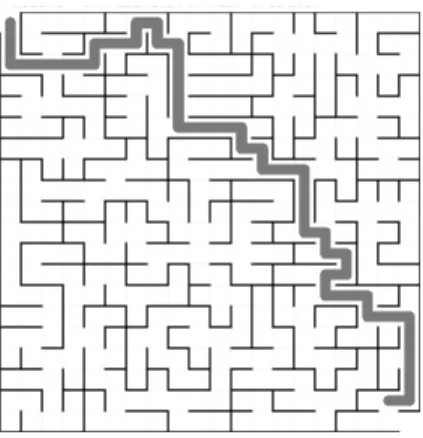
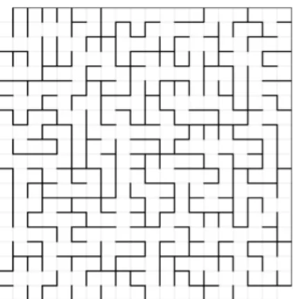
In the case of a road, this can be the name of the road or its length. It works, like Prim, by placing all vertices in a minimum priority queue, where the queue metric for each vertex is the length of the path connecting the vertex to the source. An application of the Dijkstra is solving a maze as constructed when discussing incoherent sets.
Given a maze of cells, path[i] gives us a tuple(j,d) where is the number of steps for the shortest path to reach the origin (0) and is the ID of the next cell along this path.
Greedy algorithms
- Huffman encoding
- Longest common subsequence
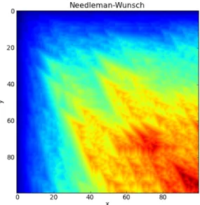
- Needleman–Wunsch
- Continuous Knapsack
- Discrete Knapsack
We then associate with the root node the frequency of the character representing the tree. At this point, we associate a series of bits with each node of the tree. Given two sequences of characters S1 and S2, the problem is to determine the length of the longest common subsequence (LCS) that is a subsequence of both S1 and S2.
From this we can observe the following simple fact: if both strings start with the same letter, it is always safe to choose that initial letter as the first character of the subsequence.
Artificial intelligence and machine learning
- Clustering algorithms
- Neural network
- Genetic algorithms
Hierarchical clustering only requires the idea of a distance between points for some points. Figure 3.7: Number of clusters found as a function of the distance limit. ordered into the layers with one input layer of neurons connected only to the input and the next layer. Each neuron is defined by a set of parametersa that determined the relative weight of the input signals.
Therefore, the DNA of the offspring is as good as the average of their parents.

Long and infinite loops
- P, NP, and NPC
- Cantor’s argument
- Gödel’s theorem
The only trick is finding a proper mating algorithm that preserves some of the fitness traits of the parents in their offspring's DNA. Assume that these real numbers are countable. to associate each of them with an integer. here represent a decimal digit of a real number). where the first decimal digit differs from the first decimal digit of the first real number of the table 3.99, the second decimal digit differs from the second decimal digit of the second real number of the table 3.99, and so on and so forth for all . Gödel used a similar diagonal argument to prove that there are as many problems (or theorems) as real numbers and as many algorithms (or proofs) as natural numbers [33].
Because there are more of the former than the latter, it follows that there are problems for which there is no corresponding solution algorithm.
Well-posed and stable problems
A problem is said to be best if its solution is not only continuous, but also weakly sensitive to input data. A problem with a low condition number is said to be well conditioned, while a problem with a high condition number is said to be badly conditioned. We say that a problem characterized by a function f is well conditioned in a domain D if the condition number is less than 1 for each entry in the domain.
If a problem is well conditioned for all inputs in a domain, it is also stable.
Approximations and error analysis
- Error propagation
We could choose a more accurate instrument, but it would not change the fact that different measures will yield different values according to the resolution of the instrument. Now let's consider a system that, given an inputx, produces the output y; x and y are physical quantities that we can measure, albeit only with a finite resolution. We can model the system with a function f such that y= f(x) and, in general, f is unknown.
We can replace the "true" value for the input with our best guess, ¯x, and its associated uncertainty, δx.
Standard strategies
- Approximate continuous with discrete
- Replace derivatives with finite differences
- Replace nonlinear with linear
- Transform a problem into a different one
- Approximate the true result via iteration
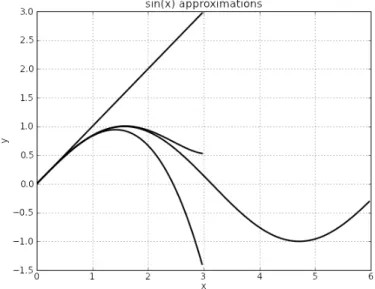
- Taylor series
- Stopping Conditions
We can easily implement the concept of a numerical derivative in code by creating a function D that takes a function f and returns the function. In this case, we can use the following relations to reduce the computation of sin(x) for large x to sin(x) for 0< x <1. In general, we can repeat the process of finding corrections and approximating the true result.
We also need to detect which of the two conditions causes the algorithm to stop running and return, so that we can estimate the uncertainty in the result.
Linear algebra
- Linear systems
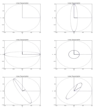
- Examples of linear transformations
- Matrix inversion and the Gauss–Jordan algorithm
- Transposing a matrix
- Solving systems of linear equations
- Norm and condition number again
- Cholesky factorization
- Modern portfolio theory
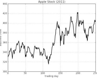
- Trading and technical analysis
- Eigenvalues and the Jacobi algorithm
- Principal component analysis
Figure 4.3: Example of the effect of different linear transformations on the same set of points. In fact, any linear combination of the tangency portfolio with a risk-free asset (putting money in the bank) has the same Sharpe ratio. For any target risk, one can find a linear combination of the risk-free asset and the tangent portfolio that has a better Sharpe ratio than any other possible portfolio that includes the same assets.
Figure 4.5: Eigenvalues of the correlation matrix for 20 of the S&P100 stocks, sorted by their size.
Sparse matrix inversion
- Minimum residual
- Stabilized biconjugate gradient
The defocusing operation can be modeled as a first approximation with a linear operator that acts on the "true" image, x, and turns it into an "out of focus" image, y. The larger the values of β and α are, the more out of focus the original image is. Figure 4.6: An out-of-focus image (left) and the original image (image) calculated from the out-of-focus using sparse matrix inversion.
When the Hubble telescope was first put into orbit, its mirror was not installed correctly, causing the telescope to take pictures out of focus.
Solvers for nonlinear equations