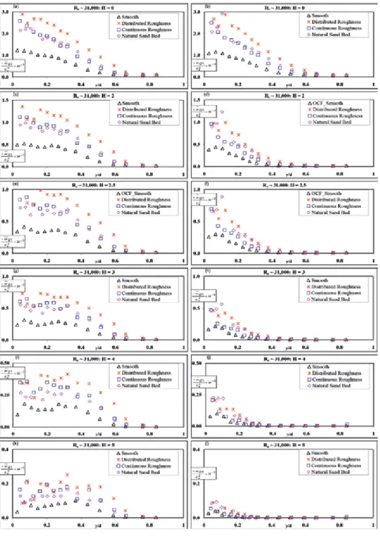
For the second problem, a model of the interaction of the boundary layer and the discharge is proposed. The purpose of this study [1] is to explain how roughness and Reynolds number affect flow characteristics in open channel flow (OCF).
Introduction
Such models are based on mixing the laminar and turbulent regions of the flow field by introducing intermittence equations into the turbulence equations. Therefore, transition modeling as part of turbulence has always stood at the heart of the matter in terms of turbulence modeling. Next in the series of increasing complexity comes the class of the so-called correlation-based transition models [1].
These models are based on the basic approach of mixing the laminar and turbulent regions of the flow field by introducing discontinuity equations into the turbulence equations. Following the success of "nonlocal" transition models using discontinuous transport equations, including experimental correlations, a number of new methods have been developed [10, 11], named as local correlation-based transition models (LCTM) by Menter et al.
Low Reynolds number turbulence models
These methods take advantage of the random ability of the wall damping terms to mimic some of the effects of transition. 12], variations of the k-kL-ω models of Walters and Leylek [13] and Walters and Cokljat [14], and the k-ω-γ model of Fu and Wang [15] with super/hypersonic flow applications. In the following, a brief overview of the transition modeling is made covering the practical applications of a range of models currently used in industrial design aerodynamics.
In this method, the Orr-Sommerfeld eigenvalue equations are solved using previously obtained velocity profiles over a surface in order to calculate the local instability amplification rates of the most unstable waves for each profile. The transition is said to occur when the value of the amplification factor exceeds a threshold value N.
Intermittency equation transition models
This model is based on the understanding that free-stream turbulence is the cause of high-amplitude current fluctuations in the pre-transitional boundary layer, and these fluctuations are quite distinct from classical turbulence fluctuations. In the application, the output term of the underlying turbulence model is smoothed until a significant amount of turbulent viscosity is generated, and the damping effect of the transition model will be disabled after this point. Furthermore, in the formulation of the B-C model, the free stream turbulence intensity parameter is present only as a function of the Reynolds number of the critical momentum thickness which makes the model calibration quite easy for various problems.
After a point where the starting criteria are ensured, the damping effect is controlled by the intermittence function γBC,. Inspection of the Term2 equation with the νBC relation shows that the regions close to the wall are inversely related and the damping effect of the transition model would be disabled inside the boundary layer.
Two- and three-dimensional test cases for low to high speeds Some outstanding test cases that make a good platform for measuring novel
Low speed flat plate test cases
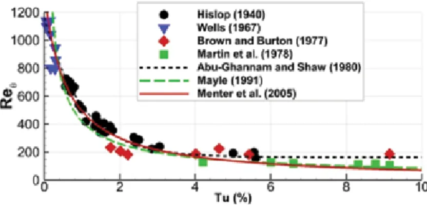
In fact, Term1 checks for the transition start point by comparing the locally calculated Reθ with the experimentally obtained critical momentum thickness Reynolds number Reθc. Two- and three-dimensional test cases for low to high speed Some outstanding test cases that make a good platform to measure novel. In the S&K calibration case, the B-C model shows good agreement with experiment for the transition onset similar to other methods.
For the T3C2 case, although the B-C model predicted a good starting point of the transition, it is observed that the turbulent stress rises abruptly after the onset. For the T3C3 case, the γ-Reθ model [11], the k-kL-ω model [14] and the WA-γ model [24] are observed to outperform the other models, as the prediction of the B–C model shows an early transition onset, while the one equation γ model [22] predicts a rather late transition onset.
Airfoil and turbomachinery test cases .1 S809 airfoil
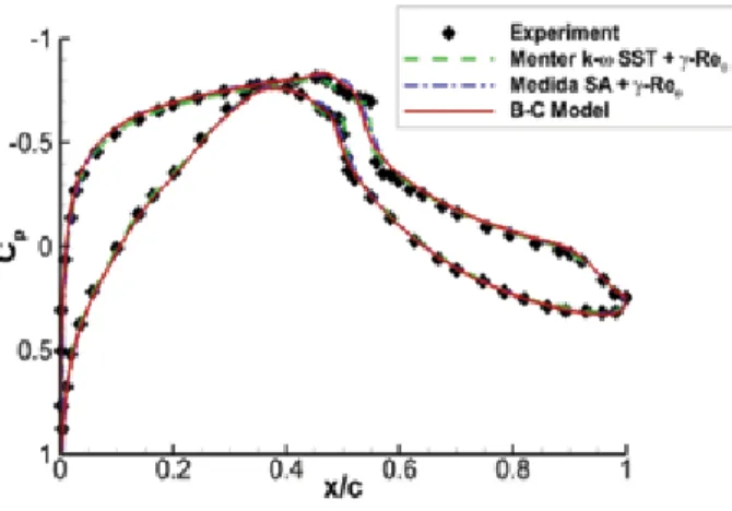
In the experiment, the flow conditions correspond to a Reynolds number of nearly 91,000 based on the chord length of the T106 airfoil and the inlet velocity. Comparison of the experimental and numerical pressure coefficient distributions for the T106 cascade for the steady case is depicted in Figure 7. Looking at Figure 7, it is observed that the separation bubble on the blade predicted by the B-C model and the two-equation γ-Reθ model is slightly smaller in size than the experimentally measured bubble.
The wing is mounted to the tunnel wall with a smooth transition area and the angle of attack is set at 2°. Finally, to highlight the difference between the fully turbulent and the transient solutions, comparison of the skin friction coefficients at 80% span.
Conclusions
1] two-equation γ-Reθ transition model summarizes to a total of four-equation model by incorporating the two-equation k-ω SST turbulence model of Menter et al. Similarly, Medida [31] developed a three-equation S-A-γ-Reθ transition model that is a sum of the Menter et al. 19] with the introduction of the algebraic Bas-Cakmakcioglu (B-C) model by including an algebraic γ-function with the one-equation S-A turbulence model [28].
Comparison of skin friction coefficients predicted by the S-A turbulence model and the B-C transition model at 80% span on the DLR-F5 wing. The quality of the model depends on the similarity between the laboratory generated flow and the atmospheric flow.
Boundary layer flows at the UNNE wind tunnel
The boundary layer obtained with empty tunnel
The uniformity of the flow corresponding to the empty boundary layer wind tunnel has been evaluated previously to implement physical models for turbulent flows. Finally, the longitudinal component of the turbulence spectrum is obtained from the boundary layer flow and from the uniform flow. The depth of the boundary layer is approx. 0.3 m, and a good uniformity can be observed from the vertical velocity distributions.
A maximum deviation from the average velocity of approximately 3% is verified outside the boundary layer by taking the velocity in the middle of the channel as reference. The value of Reynolds number calculated with the hydraulic diameter of the test section was 3.67 × 10⁶.
Full-depth simulation of the atmospheric boundary layer
Dimensionless velocity profiles measured with the empty tunnel along a vertical line in the center of the test section rotary table (see reference [8]) and at positions 0.6 m to the right and left of this line are shown in Figure 2. The complete boundary layer thickness of the ABL is simulated when a full-depth simulation is developed. Measurements of the mean velocity distribution were made along a vertical line on the center of the rotary table and along lines 0.30 m to the right and left of this line.
There is a good similarity between the three measured velocity profiles and the value of the exponent α obtained by fitting Eq. An important feature of the spectra is the presence of a clear region of the Kolmogor inertial subregion.
Part-depth simulation of the atmospheric boundary layer
The comparison of the results obtained by the atmospheric boundary layer simulations is made by means of dimensionless variables of the auto-spectral density and of the frequency using the von Kármán spectrum (Eq. Two Irwin-type generators separated at 1.5 m were used to simulate the partial-depth boundary layer by means of the Standen method [10]. Vertical velocity distribution and the corresponding log graph representation to verify the extension of the logarithmic behavior are shown in Fig. 8.
Dimensionless spectra obtained at different heights for the part-depth boundary layer simulation and the von Kármán spectrum. Dimensionless spectral comparison indicates a shift of the experimental peak to low frequencies with respect to the von Kármán spectrum.
Boundary layer flows at the UFRGS wind tunnel
Simulation of atmospheric boundary layers with different velocities Four perforated spires, a barrier, and surface roughness elements were used to
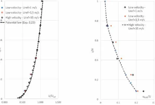
Vertical mean velocity and turbulence intensity profiles measured for subdepth boundary layer simulation. The Joaquim Blessmann boundary layer wind tunnel at the Laboratório de Aerodinâmica das Construções in UFRGS, Brazil, is a closed return loop and has a cross section of 1.30 m × 0.90 m at the downstream end of the main working section, which is 9.32 m 10 (figure). Velocity and longitudinal velocity fluctuations were measured using a TSI hot-wire anemometer along a vertical line on the center of the rotary table located downstream of the working section.
Power spectra of the velocity fluctuations obtained at two different positions, z = 0.15 and 0.35 m with low velocities Uref = 1 and 3.5 m/s, respectively, are presented in Figure 13. Poor definition of Kolmogorov's inertial subrange is observed for the spectra measured at velocity Uref = 1 m/s.
Analysis of the model scale factor
These profiles are compared with the values obtained with the highest achievable average speed in the wind tunnel (Uref ≈ 35 m/s). Turbulence intensity values corresponding to 3.5 m/s are slightly higher than those obtained at high speed, which is a behavior often observed at low speeds. For measurements at speed Uref = 1 m/s compared to 3.5 and 35 m/s cases even larger deviations can be observed which can be attributed to extremely low speed.
It is worth noting that at these velocity magnitudes, the relative errors affecting the hot-wire anemometer technique are larger than for high-velocity measurements. The sampling series used for the spectral analysis were obtained with an acquisition frequency of 1024 Hz.
Recent applications of simulated boundary layer flows
- Wind tunnel study of the aerodynamic loads on a low structure
- Aerodynamic analysis of cable-stayed bridges
- Study of atmospheric dispersion by means of scale model
- Wind tunnel tests of the flow in the wake of wind turbines
Jacek A study of the wind loads on a high-rise building was realized in Prof. The high-rise scale model in the test section of the UNNE wind tunnel and details of the fluctuating local pressure. The determination of the critical speed is very important in the design of cable-stayed bridges.
Figure 16, left, shows a picture of a 1:60 dynamic cross-sectional model installed in the test section of the Prof. wind tunnel. Sectional model and fully aeroelastic model of the Octávio Frias de Oliveira suspension bridge in the wind tunnel of Prof.
Concluding remarks
In these experiments, the adequacy of spectral technique and changes in the turbulence spectral composition of the incident wind and the coil were analyzed [25]. Launch of a space vehicle at the ACL, Maranhão, Brazil, and simulation of the dispersion process in the wind tunnel of the LAC/UFRGS. Vertical profiles of dimensionless mean longitudinal velocity and spectral comparison of the incident wind and the streamflow at z = 225 mm.
Finally, a recent wind tunnel study of the flow in the wake of wind turbines is presented. Determination of the model scale factor in wind tunnel simulations of the adiabatic atmospheric boundary layer.
Experimental setup
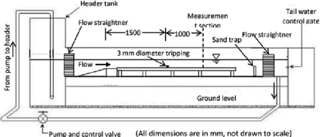
The design and equipment of the hydrodynamic flume allowed the flow rate and water depth to be controlled within wide limits. Inside the system of oval dimples and in their close wake, 12 sensors of pressure fluctuations were used (Figure 2b). The degree of flow turbulence in the hydrodynamic trough did not exceed 10% for the velocity range of 0.03 to 0.5 m/s.
The measurement error of the average parameters of the velocity and pressure fields did not exceed 10%. The measurement error of the spectral components of the velocity fluctuations did not exceed 1 dB, and the pressure and acceleration fluctuations—.
Research results
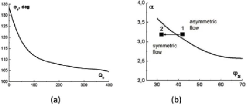
A spectral analysis of the wall pressure fluctuations on the streamlined surfaces of the oval dimples and plate was performed. Power spectral densities of the wall pressure fluctuations inside (a) and near (b) the oval dimple for the Reynolds number Re X = 200,000. The smallest spectral levels are generated in the forward spherical part of the dimple (curve 2).
Power spectral densities of the wall pressure fluctuations inside (a) and near (b) the oval dimple for the Reynolds number Re X = 400,000. In the central part of the oval dimple system at a distance 2 d from the dimples, discrete peaks appear in the spectral levels of wall pressure fluctuations. Influence of the deep spherical dimple on the pressure field below the turbulent boundary layer.
It was found that the influence of the shape of the roughness on the performance of the corrugated channels is small.