Computational Models in Engineering

(1)

Computational Models in Engineering

Edited by Konstantin Volkov

The accurate prediction of multi-physical and multi-scale physical/chemical/mechanical processes in engineering remains a challenging problem despite considerable work

in this area and the acceptance of finite element analysis and computational fluid dynamics as design tools. This book intends to provide the reader with an overview of the latest developments in computational techniques used in various engineering disciplines. The book includes leading-edge scientific contributions of computational and

applied mathematics, computer science and engineering focusing on the modelling and simulation of complex engineering systems and multi-physical/multi-scale engineering problems. The following topics are covered: numerical analysis and algorithms, software development, coupled analysis, multi-criteria optimization as they applied to all kinds of applied and emerging problems in energy systems, additive manufacturing, propulsion

systems, and thermal engineering.

Published in London, UK

ISBN 978-1-78923-869-3

Computational Models in Engineering

(2)

(3)

Computational Models in Engineering

Edited by Konstantin Volkov

Published in London, United Kingdom

(4)

(5)

(6)

http://dx.doi.org/10.5772/intechopen.77484 Edited by Konstantin Volkov

Contributors

Faham Tahmasebinia, Chengguo Zhang, Ismet Canbulat, Samad M.E. Sepasgozar, Onur Vardar, Serkan Saydam, Chen Chen, Jeongho Kim, Ganesh Anandakumar, Andrey Kurkin, Andrey Kozelkov, Valentin Efremov, Sergey Dmitriev, Vadim Kurulin, Dmitry Utkin, Md Sakib Hasan, Mst Shamim Shawkat, Sherif Amer, Nicole McFarlane, Syed Islam, Garrett Rose, Mohammed Albadi, Yuri Menshikov, Dimitris Spiridakos, Nicholaos Markatos, Despoina Karadimou

The rights of the editor(s) and the author(s) have been asserted in accordance with the Copyright, Designs and Patents Act 1988. All rights to the book as a whole are reserved by INTECHOPEN LIMITED.

The book as a whole (compilation) cannot be reproduced, distributed or used for commercial or non-commercial purposes without INTECHOPEN LIMITED’s written permission. Enquiries concerning the use of the book should be directed to INTECHOPEN LIMITED rights and permissions department (permissions@intechopen.com).

Violations are liable to prosecution under the governing Copyright Law.

Individual chapters of this publication are distributed under the terms of the Creative Commons Attribution 3.0 Unported License which permits commercial use, distribution and reproduction of the individual chapters, provided the original author(s) and source publication are appropriately acknowledged. If so indicated, certain images may not be included under the Creative Commons license. In such cases users will need to obtain permission from the license holder to reproduce the material. More details and guidelines concerning content reuse and adaptation can be found at http://www.intechopen.com/copyright-policy.html.

Notice

Statements and opinions expressed in the chapters are these of the individual contributors and not necessarily those of the editors or publisher. No responsibility is accepted for the accuracy of information contained in the published chapters. The publisher assumes no responsibility for any damage or injury to persons or property arising out of the use of any materials, instructions, methods or ideas contained in the book.

First published in London, United Kingdom, 2020 by IntechOpen

IntechOpen is the global imprint of INTECHOPEN LIMITED, registered in England and Wales, registration number: 11086078, 7th floor, 10 Lower Thames Street, London,

EC3R 6AF, United Kingdom Printed in Croatia

British Library Cataloguing-in-Publication Data

A catalogue record for this book is available from the British Library Additional hard and PDF copies can be obtained from orders@intechopen.com Computational Models in Engineering

Edited by Konstantin Volkov p. cm.

Print ISBN 978-1-78923-869-3 Online ISBN 978-1-78923-870-9 eBook (PDF) ISBN 978-1-78985-400-8

(7)

Selection of our books indexed in the Book Citation Index in Web of Science™ Core Collection (BKCI)

Interested in publishing with us?

Contact book.department@intechopen.com

Numbers displayed above are based on latest data collected.

For more information visit www.intechopen.com

4,700+

Open access books available

Countries delivered to

151 12.2%

Contributors from top 500 universities Our authors are among the

Top 1%

most cited scientists

120,000+

International authors and editors

135M+

Downloads

We are IntechOpen,

the world’s leading publisher of Open Access books

Built by scientists, for scientists

(8)

(9)

Meet the editor

Dr. Volkov is a senior lecturer in thermofluids at the Kingston University (London, UK). He holds a PhD in fluid mechanics.

After completion of his PhD, Dr Volkov worked at the Bal- tic State Technical University (Russia), University of Central Lancashire (UK), and University of Surrey (UK). His areas of expertise cover multidisciplinary areas: from design and optimization of energy systems to fundamental problems focused on modelling and simulation of turbulent multi-phase flows. He is a Chartered Engi- neer and member of the Institute of Physics, Institution of Mechanical Engineers, Combustion Institute, and Higher Education Academy. He is the author of more than 120 scientific papers and a member of editorial boards and scientific commit- tees of a number of journals and conferences.

(10)

(11)

Preface XIII

Chapter 1 1

Technology of 3D Simulation of High-Speed Damping Processes in the Hydraulic Brake Device

by Valentin Efremov, Andrey Kozelkov, Sergey Dmitriev, Andrey Kurkin, Vadim Kurulin and Dmitry Utkin

Chapter 2 17

Three-Dimensional Finite Element Analysis for Nonhomogeneous Materials Using Parallel Explicit Algorithm

by Ganesh Anandakumar and Jeongho Kim

Chapter 3 35

A New Concept to Numerically Evaluate the Performance of Yielding Support under ImpulsiveLoading

by Faham Tahmasebinia, Chengguo Zhang, Ismet Canbulat, Samad M.E. Sepasgozar, Onur Vardar, Serkan Saydam and Chen Chen

Chapter 4 47

Criteria for Adequacy Estimation of Mathematical Descriptions of Physical Processes

by Yuri Menshikov

Chapter 5 67

Power Flow Analysis by Mohammed Albadi

Chapter 6 89

Modeling Emerging Semiconductor Devices for Circuit Simulation by Md Sakib Hasan, Mst Shamim Ara Shawkat, Sherif Amer, Syed Kamrul Islam, Nicole McFarlane and Garrett S. Rose

Chapter 7 115

Mathematical Modeling of Aerodynamic Heating and Pressure Distribution on a 5-Inch Hemispherical Concave Nose in Supersonic Flow

by Dimitrios P. Spiridakos, Nicholas C. Markatos and Despoina Karadimou

(12)

(13)

In many fields, modelling and simulation are integral and therefore essential to business and research. Modelling and simulation provide the capability to enter fields that are either inaccessible to traditional experimentation or where carrying out traditional empirical inquiries is prohibitively expensive. The role of modelling and simulation in engineering and various applications such as computational fluid dynamics, finite element analysis, and others has been underestimated for a long time. However, with a growing complexity of application scenarios as well as numerical algorithms and hardware architectures, the need for sophisticated methods from numerical analysis and computer science has become more important. The growth in computing power has revolutionized the use of realistic mathematical models in science and engineering, and numerical analysis is required to implement these detailed models of the world.

A computer simulation is the execution of a model, represented by a computer program that gives information about the system being investigated. The simulation approach of analyzing a model is opposed to the analytical approach, where the method of analyzing the system is purely theoretical. As this approach is more reliable, the simulation approach gives more flexibility and convenience. Modelling and simulation offer people the chance to develop an understanding of their problem domain by building a simulation of the problem space in which they are interested.

The modelling and simulation identify more key stages in a successful simulation cycle: implementation, exploration and visualization, validation, and embedding.

The book provides and discusses different examples from engineering, as well as where and how numerical methods contribute to more efficient simulation environments. There are 7 chapters in the book, covering different aspects of modelling and simulation in engineering and technology.

In Chapter 1, a three-dimensional simulation technology for physical processes in concentric hydraulic brakes with a throttling-groove partly filled hydraulic cylinder is considered. The technology is based on the numerical solution of a system of Navier-Stokes equations. Free surface tracking is provided by the volume of fluid method. The results of hydraulic brake simulations in the counter-recoil regime are reported and compared to experimental data. The performance of the hydraulic brake is studied as a function of the fluid mass and firing elevation of the gun.

Chapter 2 addresses the behavior of functionally graded solids under dynamic impact loading within the framework of linear elasticity using the parallel explicit algorithm. Numerical examples are presented that verify the dynamic explicit finite element code and demonstrate the dynamic response of graded materials. A three- point bending beam made of epoxy and glass phases under low velocity impact is studied. Finite element modeling and simulation discussed herein can be a critical tool in helping to understand the physics behind the dynamic events.

(14)

Chapter 3 discusses the case studies that revealed premature failures of stiffer elements prior to utilising the full capacity of more deformable elements within the same system. From a design perspective, it is important to understand that the dynamic-load capacity of a ground support system depends not only on the capacity of its reinforcement elements but also, and perhaps most importantly, on their compatibility with other elements of the system and on the strength of the connec- tions. The failure of one component of the support system usually leads to the failure of the system.

Chapter 4 estimates criteria for mathematical descriptions in the form of ordinary differential equations. Adequate mathematical descriptions can increase the objec- tivity of the results of mathematical modeling for future use. These descriptions make it possible and reasonable to use the results of mathematical modeling to optimize and predict the behavior of physical processes. Interrelations between criteria are considered. The proposed criteria are easily transferred to mathematical descriptions in algebraic form.

In Chapter 5, the power flow model of a power system is built using the relevant network, load, and generation data. Outputs of the power flow model include voltages at different buses, line flows in the network, as well as system losses. These outputs are obtained by solving nodal power balance equations. Since these equations are nonlinear, iterative techniques are commonly used to solve this problem.

The chapter will provide an overview of different techniques used to solve the power flow problem.

Chapter 6 shows how different approaches can be adopted to model three emerging semiconductor devices namely, silicon-on-insulator four gate transistor, single photon avalanche diode, and insulator-metal transistor device.

In Chapter 7, the results of numerical simulation of heat transfer on a 5-inch hemispherical concave nose at a Mach number of 2 are reported and compared with the available experimental data. Different turbulence models and different

discretization schemes are also examined.

The book promotes open discussion between research institutions, academia, and industry from around the globe on research and development of enabling technol- ogies. The book covers many aspects of theory and practice, which deliver essential contributions and provide their input and support to the cooperative efforts.

Dr. Konstantin Volkov MEng. MSc. PhD. DSc. CEng. MIMechE. MinstP. FHEA., Department of Mechanical and Automotive Engineering, School of Engineering and the Environment, Faculty of Science, Engineering and Computing, Kingston University, London, United Kingdom

(15)

Technology of 3D Simulation of High-Speed Damping Processes in the Hydraulic Brake Device

Valentin Efremov, Andrey Kozelkov, Sergey Dmitriev, Andrey Kurkin, Vadim Kurulin and Dmitry Utkin

Abstract

This chapter describes a three-dimensional simulation technology for physical processes in concentric hydraulic brakes with a throttling-groove partly filled hydraulic cylinder. The technology is based on the numerical solution of a system of Navier–Stokes equations. Free surface tracking is provided by the volume of fluid (VOF) method. Recoiling parts are simulated by means of moving transformable grids. Numerical solution of the equations is based on the finite-volume

discretization on an unstructured grid. Our technology enables simulations of the whole working cycle of the hydraulic brake. Results of hydraulic brake simulations in the counter-recoil regime are reported. The results of the simulations are compared with experimental data obtained on JSC“KBP”test benches. The calculated and the experimental sets of data are compared based on the piston velocity as a function of distance. The performance of the hydraulic brake is studied as a function of the fluid mass and firing elevation of the gun.

Keywords:hydraulic brake, Navier-stokes equations, multi-phase flow, volume of fluid, moving rigid body, turbulent flow

1. Introduction

This chapter describes our three-dimensional simulation technology for physical processes in hydraulic brakes with a throttling-groove partly filled hydraulic cylinder. The technology is based on the numerical solution of a system of Navier- Stokes equations with an additional transport equation to track the working fluid/

free volume interface by the volume of fluid (VOF) method [1, 2]. As a solver, we use an iterative algorithm, PISO [1, 3], combined with a SLAE solver based on the algebraic multigrid method [4]. To improve the accuracy of solution, we use interface capturing schemes, HRIC [1, 4], near the interface between the phases.

Moving parts are simulated by means of moving deforming meshes [5], the motion of which is represented in the initial equations with the Lagrange-Eulerian approximation [6]. Our technology enables modeling of the whole working cycle of the hydraulic brake.

To demonstrate the performance of our technology, we are considering simulation of a hydraulic brake with a throttling-groove partly filled hydraulic cylinder. The simulation outputs are compared with experimental data obtained on the

(16)

test benches at JSC“KBP.”The calculated and the experimental sets of data are compared based on the piston velocity as a function of displacement. The performance of the hydraulic brake is studied as a function of the fluid mass and hydraulic brake angle.

2. Problem definition

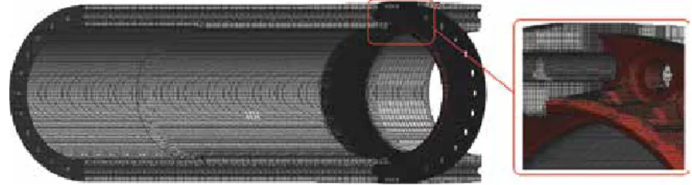
The hydraulic brake serves to absorb the energy of moving parts. Its structure consists of a case with a grooved inner surface, a ring piston mounted directly on the outer surface of the barrel and having holes matching the guide rods with stranded counter-recoil springs uniformly distributed around the barrel in the hydraulic brake chamber, and front and rear packings with circular-cross-section rubber O-rings to seal the hydraulic brake chamber filled with hydraulic fluid (Figure 1).

The hydraulic brake starts to react as soon as there is no more free space in the recoil chamber (space between the piston and the rear packing); the fluid is sprinkled through the gaps from the recoil chamber to the counter-recoil chamber (space between the piston and the front packing) at a growing rate and stops the moving parts.

Recoil of the moving parts is countered by the energy stored by the counter- recoil springs while braking. In the counter-recoil phase, the fluid from the counter- recoil chamber is sprinkled through the gaps into the recoil chamber providing the

Figure 1.

(a) General layout of the hydraulic brake: (a) general layout (1—hydraulic fluid cylinder with guides and springs, 2—case, 3—piston, 4—packings); (b) general layout without case (5—guides); and (c) piston;

(b) schematic of operation.

(17)

required counter-recoil braking law. Both for recoil and for counter recoil, the areas of fluid flow in the hydraulic brake are generated by the gaps between the piston and the grooved case surface defining the law of motion, and between the piston holes and the guide rods.

Numerical simulation of the hydraulic brake includes the following physical processes: turbulent flow of fluid encountering sudden contractions, expansions, and axisymmetric gaps; multi-phase flow with different equations of state (it is reasonable to use constant-density approximation for fluid and perfect gas law for air); and flow with moving solids.

The scope of this work included the development of a mathematical model and numerical method to simulate these physical processes.

3. Mathematical model and numerical scheme

Simulation of hydraulic brake operation involves multi-phase flow simulation with two phases. Each phase can have its individual equation of state. Let us assume that the flow is isothermal within one operation cycle and that the phases have the same field of velocity. These assumptions allow us to construct our numerical model using the VOF method [1, 7]. Considering the assumptions above, let us describe the flow of matter by a system of equations, comprised of the mass and momentum equations and the volume fraction transfer equation:

∂ρ

∂tþ ∂

∂x_iðρuiÞ ¼0,

∂ρui

∂t þ ∂

∂xi�ρuiuj�

¼ �∂p

∂xiþ ∂

∂xiτijþρg_i,

∂ρ_ξα_ξ

∂t þ ∂

∂x_i uiρ_ξαξ

� �

¼0, 8>

>>

><

>>

:

(1)

wheretis the time,u_i={u1,u2,u3} = {u,v,w} is the velocity,xiis the spatial vector component,τijis the viscous stress tensor,giis the gravity acceleration vector,ξis the phase index,αξis the volume fraction of theξ-th phase, andρis the resulting density defined as an average over all the phases:

ρ¼∑^N

ξ¼1ρ_ξαξ (2)

whereNis the number of phases.

The volume fraction transfer equation is written in terms of the transfer of the quantityαξ:

∂αξ

∂t þ ∂

∂xi�u_iα_ξ�

¼ �αξ

ρ_ξ

∂ρ_ξ

∂t þu_i∂ρ_ξ

∂xi

� �

(3) Summing Eq. (3) over all the phases and considering the equality∑_ξα_ξ¼1, we obtain the following mass equation with respect to the velocity divergence:

∂ui

∂x_i¼ �∑

ξ

αξ

ρ_ξ

∂ρ_ξ

∂t þui

∂ρ_ξ

∂x_i

� �

¼ �∑

ξ

αξ

ρ_ξ dρ_ξ

dt (4)

The momentum equation is written in a half-divergent form. This stabilizes the iterative procedure of numerical solution of this equation [3, 4]:

(18)

ρ∂ui

∂t þ ∂

∂xjρuiuj

�ui

∂

∂xjρuj

¼ �∂p

∂xiþ∂τij

∂xjþρg_i (5) An important feature of this problem is that we need to consider the motion of moving parts, which travel to a distance exceeding the half length of the hydraulic brake during computation. To incorporate their motion, we decided to use a topology-preserving mesh deformation method. To prevent unnecessary cell defor- mations, the mesh nodes located at fixed elements (case and guide rods) follow the moving piston preserving their geometry. The mesh deformation was implemented by the IDW method [5].

To allow for the mesh motion in Eq. (1), we have rewritten the equations of volume fraction transfer and momentum of the phases in a moving frame of coordinate in accordance with the known law [6]:

d^∗φ dt ¼∂φ

∂t þvi

∂φ

∂xi (6)

where^d_dt^∗^φis the substantial derivativeφwith respect to the moving frame of reference andviis the mesh displacement velocity vector. Using Eq. (3), the volume fraction transfer equation can be written as:

d^∗αξ

dt þðu_i�v_iÞ∂αξ

∂x_iþαξ

∂ui

∂x_i¼ �αξ

ρ_ξ d^∗ρ_ξ

dt þðu_i�v_iÞ∂ρ_ξ

∂x_i

(7) Here^d^∗_dt^α^ξdenotes the substantial derivative on the moving mesh. The momentum equation is also defined with respect to the moving frame of reference considering Eq. (3):

ρd^∗u_i dt þ ∂

∂xjρuiuj�vj

�ui

∂

∂xjρuj�vj

¼ �∂p

∂xiþ∂τij

∂xjþρg_i (8) The mass equation is defined with respect to the velocity in the moving frame of reference:

∂ðu_i�v_iÞ

∂xi ¼ �∑

ξ

α_ξ ρ_ξ

d^∗ρ_ξ

dt þðui�viÞ∂ρ_ξ

∂xi

(9) This form of the equations is easy to implement within the framework of finite- volume discretization [8–11]. The chosen way of taking into account the mesh motion is optimal, because it does not require topology reconstruction, though conservative with respect to the major quantities.

The experimental data on the hydraulic brake operation make it possible to estimate the Reynolds number, which equals Re = 10⁵–10⁶in the cylindrical gap during recoil of the moving parts. The most reasonable way to include turbulent flow components with such a Reynolds number is to use the RANS approach based on the solution of the Reynolds-averaged system Eq. (2) [8, 9]. The averaged system of equations is closed using the SST turbulence model, which has proven its efficiency in real-life problem simulations [11–13]. In the SST model, the (k-ε) model is formulated in terms of (k-ω) and is focused on resolving small-scale turbulence in the outer flow region. A (k-ω) model intended to describe large-scale turbulence is used in the boundary layer. The combination of these models together is carried out with the help of a function that ensures the proximity of the total model to the (k-ε) model far from the solid walls and to the (k-ω) model in the near-wall flow area.

(19)

The resulting system of equations is solved by numerical integration on the finite-volume mesh. The relationship of pressure and velocity while solving Eq. (1) is determined by the SIMPLE algorithm [2]. The SIMPLE algorithm allows to find the pressure field for closure of the continuity equation. Let us write the equation of conservation of momentum at time discretization according to the Euler scheme:

ρu^nþ1_i �u_i^j Δt þρ ∂

∂xj�u^nþ1_i uⁿ_j�

¼ �∂p^nþ1

∂xi þ ∂

∂xj�τ^nþ1_ij �

(10) wherenis the solution from the previous iteration, andjis the solution from the previous time step. To solve this equation, the pressure and velocity are supposed to have the form:

u^nþ1_i ¼uⁿ_i þu^∗_i,

p^nþ1¼pⁿþαpðp^nþ1�pⁿÞ ¼pⁿþαpδp^nþ1: (

(11) Here 0≤αp≤1 is the parameter of relaxation.

Substitution of the first expression in Eq. (11) into Eq. (10) yields a preliminary estimate of the velocity value in the next step from the equation:

ρu^∗_i Δtþρ ∂

∂x_j�u^∗_iuⁿ_j�

� ∂

∂x_j� �τ^∗_ij

¼ρu_i^j Δt�∂pⁿ

∂x_i (12)

The molecular and turbulent components of the tensor of tangential stress in Eq. (12) are also calculated usingu^∗_i. In the second stage, the full speed value at the (n+ 1)th iteration is calculated by adjustment using the correction to pressure:

u^nþ1_i ¼u^∗_i �Δt∂ðδp^nþ1Þ

∂xi (13)

The pressure correction is found from Eq. (13) using the continuity condition foru^nþ1_i . Taking the derivative of both sides of Eq. (13), we obtain the Poisson equation for pressure:

∂

∂x_i

∂ðδp^nþ1Þ

∂x_i

� �

¼ 1 Δt

∂u^∗_i

∂x_i (14)

This iterative procedure allows to obtain fields of velocity and pressure satisfy- ing the system of Eq. (1).

Discretization of the equations is performed by a finite-volume technology. Let us show it on the example of the equation of transfer of a scalar quantityφ:

∂ρφ

∂t þ ∂

∂xj�ρφuj�

¼ ∂

∂xjτjþQ ,τj¼μ∂φ

∂xj (15)

The time discretization of Eq. (15) can be carried out using one of the known schemes, for example, the Euler scheme, which is used in the work to solve non- stationary problems using the RANS approach:

ρ^jþ1φ^jþ1�ρ^jφ^j

Δt þ ∂

∂xj�ρφuj�

� ∂

∂xjτj�Q

� �_jþ1

¼0 (16)

Here j is the number of the time step.

(20)

Let us integrate Eq. (16) over volume and proceed to integration over the area for the convective and diffusion terms:

ð

Vp

ρ^jþ1φ^jþ1�ρ^jφ^j

Δt dVþ

þ

Sp

ρφu_jdS_j� þ

Sp

μ∂φ

∂xjdS_j� ð

Vp

QdV¼0 (17)

For approximation on a finite-volume grid, the convective term can be written in the form:

þ

Sp

ρφujdS_j≈ ∑

k ρ_kφ_ku_j_,_kS_j_,_k≈ ∑

k ρ_kφ_kF_k (18)

whereFkis the volume flow through the facek. The value ofφkon the facekis determined by the applied convective scheme.

The discrete analog of the diffusion term can be written in the following form:

þ

Sp

μ∂φ

∂xjdS_j≈ ∑

k

μ∂φ

∂xj

� �

k

S_j_,_k¼∑

k

μ_k ∂φ

∂nk

� �

k

S_k

j j (19)

wherenkis the normal to facek.

The value of ∂^∂x^φi

� �

kon the facekis found by linear interpolation on the values of the gradient in the cells, which are determined by one of the known methods, for example, the Gauss method:

∂φ

∂xi

� �

P¼ 1

VP∑

k φ_kSk,i (20)

Using this discretization, Eq. (15) is replaced by a system of linear algebraic equations written for each calculation cell:

A_Pφ_Pþ∑

kint

A_k_intφ_M_k_int ¼R_i_,_P (21) Time discretization of the equations is performed by a three-layer second-order scheme [10]. Discretization of the convective terms in the equation of motion, equation of transfer of turbulent parameters, is performed by the upwind scheme LUD [10], and in the volume fraction transfer equation, by the HRIC scheme [1], which prevents excessive numerical diffusion of the phase interface. The force of gravity was included using a bulk force fitting algorithm [14].

These methods and models have been implemented in the software package LOGOS. LOGOS is a 3D multi-physics code for convective heat and mass transfer, aerodynamic and hydrodynamic simulations on parallel computers [11, 13–18].

LOGOS has been successfully verified and demonstrated with sufficiently high efficiency on a number of various hydrodynamic tests, including propagation of gravity waves on a free surface (tsunami) [2, 14, 18] and industry-specific simulations [11, 15]. Speedup of computations on highly parallel computers is provided by an original implementation of the algebraic multigrid method [11, 19].

4. Numerical simulation of hydraulic brake operation

Let us consider the counter-recoil phase in the operation of the hydraulic brake, when the moving parts together with the piston (seeFigure 1b) are driven by the Computational Models in Engineering

(21)

springs from their rightmost position to the leftmost one resisting the hydrodynamic force acting on the fluid side.

To solve the problem numerically, an unstructured hexahedral-dominant mesh was constructed using the pre- and post-processing tools of the LOGOS. The mesh is refined near the piston and in the gaps between the piston and the case, where the flow of fluid is particularly strong.Figure 2shows mesh fragments.

When constructing the mesh, we placed the piston in the middle between its rightmost initial and leftmost end positions of counter recoil. This minimizes mesh deformation during computation. The problem was simulated in the unsteady setup; the time step was 5�10^�4t0, wheret0is the total time of piston counter- recoil motion. The forces acting on the piston, its velocity and displacement were calculated at the end of each time step after finding the solution of the Navier– Stokes equation.

During computation, the piston together with the moving parts is accelerated by the springs and reaches its maximum velocity during the second half of its travel.

The piston then enters the grooved region of the case with a decreasing gap, as a result of which the hydrodynamic resistance grows and slows down the moving parts. The computation ends when the piston is atdm= 0.01 m from its end position, which is attributed to the maximum admissible mesh deformation in the counter-recoil chamber.

When the piston is moving, in addition to the force exerted by the springs and hydrodynamic resistance, the moving parts are exposed to friction arising in the packings, between the guides and the piston, and inside the stranded springs during their compression or tension. The resultant of the forces exerted by the springs and friction can be expanded into two components. The first does not depend on the velocity of the moving parts and can be easily measured experimentally by pulling the moving parts at a slow rate. The second depends on the velocity of the moving parts and is mostly related to friction in the turns of the stranded springs. Empirical estimates show that the second component of the resultant force can be expressed empirically as

F^din_mp¼ηuM (22)

whereuis the velocity,Mis the mass of the moving parts,ηis an empirical coefficient, which can vary in the range ofη= 0–5 s^�¹for the springs we use.

Computations were conducted withη= 0, 3, 4, and 5.Figure 3shows the field of volume fraction of the fluid at different times forη= 0 s^�1.

Att= 0.2t0, wheret0is the total time of counter recoil, a wave of fluid rises upstream of the piston. Pressure in the counter-recoil chamber grows. Air is actively bled over through the upper part of the gap. A flow of fluid emerges in the bottom part of the gap. Its rate is 10–15 times slower than the rate of the air flow (Figure 4).

Figure 2.

Mesh fragments.

(22)

As the piston continues to move, the fluid is sprinkled through the gaps at a growing rate. Att =0.95t0, most of the fluid is already pressed out of the counter- recoil chamber; it forms a nearly homogeneous gas–liquid mixture in the opposite chamber. Pressure in the counter-recoil chamber reachesP= 150P0, where P0= 1 atm is the initial pressure.

Fluid velocity in the gap grows as high asV= 50–70 m/s (Figure 5). After the fluid has flown over through the gap, the bulk gas content in the mixture increases steeply as a result of a pressure drop. This leads to a further growth of mixture velocity toV= 90 m/s (Figure 5). This effect is less pronounced in the bottom part of the gap because of the lower gas content in the mixture sprinkled through the gap.Figure 6shows a plot of piston velocity as a function of displacement for different values ofη.

On the whole, our results match the experimental data both qualitatively and quantitatively. All the simulated cases consistently predict the state of piston acceleration. In the high-velocity phase of piston motion, the parameterηstarts to play a significant role. The best agreement with experiment is provided byη= 3 s¹. This does not mean that the value above is close to the actual one, but is indicative of the fact that our numerical model, input data, and mesh are capable of describing the process of piston motion with required accuracy, if we use this value ofηin our computational model.

Figure 3.

Field of volume fraction of the fluid at different times.

Figure 4.

Field of velocity amplitude (t = 0.2 t0).

(23)

The counter-recoil phase occurs at zero angle (the hydraulic brake is placed horizontally). Let us consider the dependence of piston motion on the accuracy of horizontal positioning of the hydraulic brake. For this purpose, let us carry out calculations with anglesα= 1° andα=1°. The calculation results are shown in Figure 7.

The plots demonstrate that the piston velocity grows with increasing angle. This is quite predictable, because the amount of fluid in the counter-recoil chamber decreases as the angle increases. One should also note that the gravity force acting on the moving parts in the direction opposite to that of their motion atα> 0 or in the direction of their motion atα<0 has no measurable effect on the result.

The angle of the hydraulic brake also controls the static pressure in the counter- recoil chamber (Figure 8). The first pressure maximum is attributed to a decrease in the volume fraction of air in the counter-recoil chamber as the piston moves, and the subsequent drop, to a growth in the gap size between the piston and the grooved case region. As the angle increases, the initial amount of fluid in the counter-recoil chamber decreases, and the maximum shifts toward the range of greater piston

Figure 5.

Field of velocity amplitude (t = 0.95 t0).

Figure 6.

Piston velocity as a function of displacement.

(24)

displacements, which allows the piston to speed up to a higher velocity. This increase in the piston velocity leads to a higher pressure maximum in the region of strong slowdown (the second pressure maximum inFigure 6). Thus, an increase in the amount of fluid in the counter-recoil chamber leads to a higher and earlier first pressure maximum and a lower second pressure maximum, which is quite consistent with process physics.

The results of piston motion analysis as a function of initial fluid level in the hydraulic brake (h=h0,h=h0+ 0.01 m,h=h0–0.01 m) are shown inFigure 9.

The fluid level has a considerable effect on the piston velocity. A 1-cm increase in the level results in a 10% drop in the average piston velocity, which is explained

Figure 7.

Piston velocity as a function of piston displacement for different angles.

Figure 8.

Static pressure in the counter-recoil chamber as a function of piston displacement.

(25)

by a decrease in the force of hydrodynamic resistance acting on the moving parts.

Note that the slopes of the velocity plot are indicative of the same trend: as the fluid level in the counter-recoil chamber rises, the first pressure maximum increases and the second one decreases.

An important characteristic of the counter-recoil piston motion is piston velocity Vextrat 159 mm to the counter-recoil end (ΔZ= 153 mm), where the shell extractor is located, the performance of which depends on the velocity of the moving parts.

Another important characteristic is piston velocity close to the end positionVend, which will govern the force exerted by the piston on the packing in the counter- recoil chamber. The values of these characteristics are presented inTable 1.

The table demonstrates that a change in the fluid level within 1 cm leads to a 15%

change in the velocityVextr. A change in the angle to 1 degree results in a 5% change in the velocity. Note that the level and angle variations have a minor effect on the velocityV_end, the oscillations of which do not exceed 2–3%.

The results demonstrate that the governing quantity, which controls the performance of the hydraulic brake, is the initial fluid level in the counter-recoil chamber.

An increase in the fluid level results in a lower average piston velocity, smallerVextr

andVend, shift and rise in the first pressure maximum, and drop in the second pressure maximum. The process pattern, however, does not depend on the reason

Figure 9.

Piston velocity as a function of displacement for different fluid levels.

No. α[degree] h–h0[sm] Vextr[m/s] Vend[m/s]

1 0.0 1.0 3.64 1.74

2 0.0 0.0 3.21 1.69

3 0.0 1.0 2.78 1.65

4 1.0 0.0 3.05 1.66

5 1.0 0.0 3.38 1.72

Table 1.

Piston motion characteristics.

(26)

of the rise in the fluid level in the counter-recoil chamber: both general increase in the initial amount of fluid and negative angle of the hydraulic brake result in the same trends.

5. Conclusion

In this chapter, we have presented a three-dimensional numerical modeling technology for physical processes occurring in hydraulic brake devices. The technology is based on the numerical solution of a system of Reynolds-averaged Navier– Stokes equations. To track the free surface, we use the volume of fluid (VOF) method. Moving parts are simulated by means of moving deforming meshes.

Numerical solution of the equations is based on the finite-volume discretization, which is used to model the counter-recoil phase in hydraulic brake operation. This technology enables simulations on three-dimensional unstructured meshes. The technology is implemented based on the program package LOGOS, which provides high parallel efficiency of simulations.

The technology has been used to model the counter-recoil phase in hydraulic brake operation. Results of studying the effect of the parameter related to friction, hydraulic brake angle, and initial fluid level are reported. Our numerical experiments have demonstrated that the initial fluid level in the counter-recoil chamber is the governing quantity in hydraulic brake operation. An increase in the fluid level in the counter-recoil chamber as a result of pouring more fluid or placing the hydraulic brake at a negative angle results in the same trend in the change in pressure and its maximums.

Acknowledgements

This research has been funded by grants of the President of the Russian Federa- tion for state support of research projects by young doctors of science (MD- 4874.2018.9) and state support of the leading scientific schools of the Russian Federation (NSh-2685.2018.5), and supported financially by the Russian Founda- tion for Basic Research (project No. 16-01-00267).

Conflict of interest

The authors declare that they have no conflict of interest.

(27)

Author details

Valentin Efremov¹, Andrey Kozelkov², Sergey Dmitriev³, Andrey Kurkin³*, Vadim Kurulin²and Dmitry Utkin²

1 Joint-Stock Company“Instrument Design Bureau named after Academician A.G.

Shipunov”, Tula, Russia

2 Russian Federal Nuclear Center—All-Russian Research Institute of Experimental Physics, Sarov, Russia

3 Nizhny Novgorod State Technical University n.a. R.E. Alekseev, Nizhny Novgorod, Russia

*Address all correspondence to: aakurkin@gmail.com

by/3.0), which permits unrestricted use, distribution, and reproduction in any medium, provided the original work is properly cited.

(28)

References

[1]Ubbink O. Numerical prediction of two fluid systems with sharp interfaces [thesis]. London: Imperial College of Science, University of London; 1997 [2]Kozelkov AS, Kurkin AA, Pelinovsky EN, Tyatyushkina ES, Kurulin VV, Tarasova NV. Landslide-type tsunami modelling based on the Navier-stokes equations. Science of Tsunami Hazards.

2016;35:106-144

[3]Yatsevich SV, Kurulin VV, Rubtsova DP. On the Application of the PISO Algorithm to Molecular-Immiscible Fluid Dynamics Problems. VANT, Ser.

Matematicheskoe Modelirovanie Fizicheskikh Protsessov. Vol. 1. 2015.

pp. 16-29

[4]Khrabry AI, Smirnov EM, Zaytsev DK. Solving the convective transport equation with several high-resolution finite volume schemes. Test

computations. In: Proceedings of the 6th International Conference on

Computational Fluid Dynamics (ICCFD-6); 12–16 July 2010; Russia.

Berlin, Heidelberg: Springer-Verlag;

2011. pp. 535-540

[5]Luke E, Collins E, Blades E. A fast mesh deformation method using explicit interpolation. Journal of Computational Physics. 2012;231:586-601. DOI:

10.1016/j.jcp.2011.09.021

[6]Loitsyansky LG. Liquid and Gas Mechanics. Vol. 840. Moscow: Nauka;

1987

[7]Rusche H. Computational fluid dynamics of dispersed two-phase flows at high phase fractions [thesis]. London:

Imperial College of Science, University of London; 2002

[8]CAJ F. Computational techniques for fluid dynamics. In: Fundamental and General Techniques. 2nd ed. Vol. 1.

Berlin, Heidelberg, New York: Springer- Verlag; 1991. p. 401

[9]Fletcher CAJ. Computational techniques for fluid dynamics. In:

Specific Techniques for Different Flow Categories. Vol. 2. Berlin, Heidelberg, New York: Springer-Verlag; 1998. p. 496 [10]Jasak H. Error analysis and

estimation for the finite volume method with applications to fluid flows [thesis].

London: Imperial College of Science, University of London; 1996

[11]Kozelkov AS, Kurulin VV, Lashkin SV, Shagaliev RM, Yalozo AV.

Investigation of supercomputer capabilities for the scalable numerical simulation of computational fluid dynamics problems in industrial applications. Computational

Mathematics and Mathematical Physics.

2016;56:1506-1516. DOI: 10.1134/

S0965542516080091

[12]Menter FR, Kuntz M, Langtry R.

Ten years of experience with the SST turbulent model. In: Hanjalic K, Nagano Y, Tummers M, editors. Turbulence, Heat and Mass Transfer 4. Danbury:

Begell House Inc; 2003. pp. 625-632 [13]Kozelkov A, Kurulin V, Emelyanov V, Tyatyushkina E, Volkov K.

Comparison of convective flux

discretization schemes in detached-eddy simulation of turbulent flows on

unstructured meshes. Journal of Scientific Computing. 2016;67:176-191.

DOI: 10.1007/s10915-015-0075-7 [14]Efremov VR, Kozelkov AS, Kornev AV, Kurkin AA, Kurulin VV, Strelets DY, et al. Method for taking into account gravity in free-surface flow simulation. Computational Mathematics and Mathematical Physics. 2017;57:

1720-1733. DOI: 10.1134/

S0965542517100086 Computational Models in Engineering

(29)

[15]Deryugin YN, Zhuchkov RN, Zelenskiy DK, Kozelkov AS, Sarazov AV, Kudimov NF, et al. Validation results for the LOGOS multifunction software package in solving problems of aerodynamics and gas dynamics for the lift-off and injection of launch vehicles.

Mathematical Models and Computer Simulations. 2015;7:144-153. DOI:

10.1134/S2070048215020052 [16]Kozelkov AS, Kurkin AA, Legchanov MA, Kurulin VV, Tyatyushkina ES, Tsibereva YA.

Investigation of the application of RANS turbulence models to the calculation of nonisotermal low-Prandtl-number flows. Fluid Dynamics. 2015;50:501-513.

DOI: 10.1134/S0015462815040055 [17]Kozelkov AS, Kurkin AA, Kurulin VV, Lashkin SV, Tarasova NV, Tyatyushkina ES. Numerical modeling of the free rise of an air bubble. Fluid Dynamics. 2016;51:709-721. DOI:

10.1134/S0015462816060016 [18]Kozelkov AS, Kurkin AA, Pelinovsky EN, Kurulin VV,

Tyatyushkina ES. Numerical modeling of the 2013 meteorite entry in Lake Chebarkul, Russia. Natural Hazards and Earth System Sciences. 2017;17:671-683.

DOI: 10.5194/nhess-17-671-2017 [19]Volkov KN, Kozelkov AS, Lashkin SV, Tarasova NV, Yalozo AV. A parallel implementation of the algebraic

multigrid method for solving problems in dynamics of viscous incompressible fluid. Computational Mathematics and Mathematical Physics. 2017;57:

2030-2046. DOI: 10.1134/

S0965542517120119

(30)

(31)

Three-Dimensional Finite Element Analysis for Nonhomogeneous

Materials Using Parallel Explicit Algorithm

Ganesh Anandakumar and Jeongho Kim

Abstract

This chapter addresses the behavior of functionally graded solids under dynamic impact loading within the framework of linear elasticity using parallel explicit algorithm. Numerical examples are presented that verify the dynamic explicit finite element code and demonstrate the dynamic response of graded materials. A three- point bending beam made of epoxy and glass phases under low-velocity impact is studied. Bending stress history for beam with higher values of material properties at the loading edge is consistently higher than that of the homogeneous beam and the beam with lower values of material properties at the loading edge. Larger bending stresses for the former beam may indicate earlier crack initiation times, which were proven by experiments performed by other researchers. Wave propagation in a 3D bar is also investigated. Poisson’s ratio and thickness effects are observed in the dynamic behavior of the bar. Finite element modeling and simulation discussed herein can be a critical tool to help understand physics behind the dynamic events.

Keywords:parallel algorithm, nonhomogeneous materials, dynamic response, wave propagation

1. Introduction

Functionally graded materials (FGMs) are materials characterized by smooth variation in composition, microstructure, and properties. These materials have emerged with the need to enhance material performance and to meet specific functions and applications [1, 2]. The material gradation concept has been utilized in various applications [3–16]. The concept of FGMs has been applied to thermal barrier structures and wear- and corrosion-resistant coatings and also used for joining dissimilar materials [17]. FGMs are subjected to harsh thermal/mechanical/dynamic environments. Thin-walled plates and shells, which are used in reactor vessels, turbines, and other machine parts, are susceptible to buckling failure, large

deflections, or excessive stresses induced by thermomechanical loading. Functionally graded coatings on these structural elements may help reduce these failures [18].

The dynamic response of FGMs has been investigated [19]. Reddy and Chin [20]

carried out nonlinear transient thermoelastic analysis of FGMs by using plate elements for moderately large rotations. Gong et al. [21] studied the elastic response of

(32)

FGM shells subjected to low-velocity impact. Rousseau and Tippur [22–24] studied the dynamic fracture of a three-point bending beam made of epoxy/glass phases under low-velocity impact. Cheng et al. [25] used a peridynamic model to investigate dynamic fracture of FGMs. Lindholm and Doshi [26] looked into a slender bar with free ends and obtained a solution that is synthesized from eigenfunctions by using the principle of virtual work. Karlsson et al. [27] developed a Green’s function approach for 1D transient wave propagation in composite materials. Santare et al. [28] used graded finite elements to simulate elastic wave propagation in graded materials.

Chakraborty and Gopalakrishnan [18] developed a spectral element to study wave propagation behavior in FGM beams subjected to high-frequency impact loads.

The development of parallel computers and improvements in computer hardware has been of significant importance [29]. A dynamic event has a key characteristic that the incident pulse duration is very small in the order of microseconds that makes the frequency content of pulse very high (in the order of kHz). Thus, all the higher-order modes participate in the dynamic response, and the finite element mesh must be very fine enough to capture the small wavelengths [18]. This makes the system size enormously large. But in an explicit analysis, storage of large matrices is avoided with the added advantage of not requiring to solve linear algebraic equations [29]. Explicit methods are also conditionally stable, and so the time step size must be below a critical value that is dependent on the size of the smallest finite element [30]. Due to mesh size constraint, extremely small time steps (0.01–100μs) are needed to solve explicit problems. This can be overcome by parallel computing.

Krysl and Belytschko [30] investigated to parallelize an existing object-oriented code written in C where a Parallel Virtual Machine (PVM) was used for the necessary communication. Krysl and Bittnar [31] and Rao [32, 33] adopted the Message Passing Interface (MPI) standard for the implementation of the exchange algorithm, which is used in this chapter.

This chapter addresses the behavior of functionally graded materials under dynamic impact loading within the framework of linear elasticity using MPI-based parallel explicit algorithm. Numerical examples are presented that verify the dynamic explicit finite element code and demonstrate the dynamic response of graded materials. Finite element modeling and simulation can be a critical tool to help understand physics behind the dynamic events.

2. Finite element formulation for dynamic analysis

The governing equation for structural dynamics is given by [34]

Z

Ωðσ:δEþρu∙δu€ ÞdΩ� Z

Γ_extText∙δu dΓ¼0 (1) whereΩis domain volume,Γis the boundary with a normal vector n, u is the displacement vector, T is the traction vector,σis the Cauchy stress tensor,u is the€ acceleration vector,ρis the mass density,Γ_extrepresents the boundary surface on which external traction Textis applied, and E is the Green strain tensor. For a finite element of volumeVand surface areaS, the work balance becomes

Z δu

f g^Tf gdVF þ Z

δu

f g^Tf gdS∅ þ∑ⁿ

i¼1f gδu ^T_if gp _i

¼ Z

f gδu ^Tρf g þu€ f gδu ^Tcf g þu_ f gδε ^Tf gσ

� �

dV

(2) Computational Models in Engineering

(33)

where {F} and {Φ} represent prescribed body forces and surface tractions,f gp _i andf gδu _i�f gδε _i�

represent prescribed concentrated loads and virtual displacements and strains at a total ofnpoints, andcis a damping coefficient. The finite element discretization provides

f g ¼u ½ �Nf g;d f g ¼u_ ½ �Nn od_

;f g ¼u€ ½ �Nn od€

;f g ¼ε ½ �Bf gd (3) in which N are the shape functions, the nodal displacement vectors f gd are functions of time, and [B] is the matrix of shape function derivatives. The equation of motion is

½ �M� �D€

þ½ �C� �D_

þ½ �Kf g ¼D f gF (4) where the consistent mass (m), damping (c), and stiffness (k) matrices are given by

½ � ¼M Z

ϱð Þx ½ �N^T½ �dV CN ½ � ¼ Z

cð Þx ½ �N^T½ �dV KN ½ � ¼ Z

½ �B^T½Dð Þx �½ �dVB (5) where mass density, damping coefficient, and constitutive matrices are functions of spatial positions.

3. Explicit method, stability, and mass lumping

Dynamic response is evaluated at discrete instants of time separated by time incrementsΔt. At the nth time step, the equation of motion for linear dynamic problems is given by [34]

½ �Mf gu€ _nþ½ �Cf gu_ _nþ½ �Kf gu _n¼fF^extg_n (6) Discretization in time is accomplished using finite difference approximations of time derivatives. Explicit algorithms use a difference expression of the general form:

f gu _nþ1¼f u�f g_n;f gu_ _n;f gu€ _n;f gu _n�1;…�

(7) which contains only historical information on its right-hand side. This difference expression is combined with the equation of motion at time stepn.

The stability of the explicit finite element scheme is governed by the Courant condition [34], which provides a critical time step size beyond which the results become unstable. It is given by

Δt≤le=C_d (8)

whereleis the shortest distance between two nodes in the mesh and the dilatational wave speedCdis expressed as

C²_d¼ E xð Þð1�νð Þx Þ 1þνð Þx

ð Þð1�2νð ÞxÞρð Þx (9) SinceCdvaries due to material gradation, the desired time step for the finite element implementation is chosen based on the largest dilatational wave speed and is maintained constant throughout the simulation. The mass matrix used in the explicit method described above is typically lumped in order to avoid matrix

(34)

inversion. The HRZ technique [35] is used to lump the mass matrix in which only the diagonal terms are retained and scaled so as to preserve the total mass:

m^l_ii¼mii ∑ⁿ

j¼1mij

!,

∑ⁿ

i¼1mii

� �

(10) wherem^lis the lumped element mass matrix, m is the consistent mass matrix, andnis the number of degrees of freedom in the element.

4. Explicit parallel FEA using MPI

A master-slave approach in the parallel finite element code is used here to solve wave propagation-type problems using the Message Passing Interface (MPI) standard [36].Figure 1shows the procedure used in the parallel execution of the

Figure 1.

Time-integration procedure in the parallel execution of the explicit Newmark-βmethod [37] using MPI standard [36].

(35)

explicit Newmark-βmethod. The first step is to partition the structure (FE mesh) into number of sub-domains. The stiffness matrices are calculated for elements in the local processor. The stiffness matrix needs not be assembled in an explicit analysis as the algorithm is implemented on an element basis only. The parallel explicit time integration analysis of finite elements from onetime step to another consists in obtaining the unknown velocity and displacement of master and slaves, sending the effective force vector from slaves to the master for assembly and sending back the assembled force vector to the slaves for calculation of acceleration vector. The communication between the slaves and the master processor is done using MPI-based function calls as shown in the figure. The entire force vector at each processor is being sent to the master processor for assembly, and the master processor returns the assembled force vector to the slaves in the same manner.

These steps are repeated for the rest of the time integration. Local field quantities like element stresses and strains can be calculated separately on each processor without any communication.

5. Example 1: 3D graded beam under velocity impact

A 3D three-point bending beam under velocity impact is studied to understand the influence of material gradation on the bending behavior in a 3D space. The beam is a real FGM system made of glass/epoxy phases. The dynamic fracture experiments of the linearly graded specimens have been conducted by Rousseau and Tippur [37–40].

In this paper, we investigate the 3D dynamic behavior of a beam. Using 3D explicit finite element code, we can simulate the 3D dynamic behavior of the beam.

This 3D finite element study offers enhanced knowledge of the dynamic behavior of this material system and understanding of the stress field in homogeneous and graded materials, which help to predict fracture initiation times in various graded specimens.

Consider a three-point bending specimen under velocity impact load at the top as shown inFigure 2(a). Due to the symmetry of the geometry and the loading conditions, one-fourth of the beam is modeled as shown inFigure 2(b).

Figure 2(c)and2(d)shows the 3D FE mesh of the one-fourth model and a zoom of the FE mesh at the left bottom corner, respectively. The mesh is refined along the loaded edge with a uniform element size of 92.5μm, and the stress history at point P(0, 0.2 W) is retrieved, where W is the beam depth. Point P is of significance because it corresponds to the location of the crack tip in the dynamic fracture analysis of the cracked beam [38, 41].

Three material gradation cases are considered for the dynamic analysis of the three-point bending beam: a homogeneous beam (Homog, E2= E1), a beam stiffer at the impacted surface (StiffTop, E2> E1), and a beam softer at the impacted surface (StiffBot, E2<E1), where subscripts 1 and 2 denote bottom and top surfaces of the beam, respectively. For the graded beam, Young’s modulus (E) is varied linearly between 4 GPa and 12 GPa, and the mass density (ρ) is varied linearly between 1000 kg/cm³and 2000 kg/cm³. These material properties correspond to values used in [42]. For the homogeneous beam, the mass density (ρ) is taken as the average of the graded beam counterparts, and Young’s modulus (E) is calculated such that the equivalent E/ρvalue equals that of the graded specimen in an average sense, i.e.,

E ρ¼ 1

W Z _W

0

E yð Þ

ρð Þy dy (11)

(36)

Poisson’s ratio is 0.33 for all the three cases. The average dilatational wave speed (Cd(avg)) is defined as

CdðavgÞ ¼ 1 W

Z _W

0 Cdð Þdyy (12) where Cdis calculated assuming plane stress behavior given by

C²_d¼ E yð Þ 1�ν²ð Þy

ð Þρð Þy (13)

The dilatational wave speed (Cd) is calculated assuming plane stress behavior to compare results with those obtained by Zhang and Paulino [42]. The difference in Cd(avg)for each material gradation is marginal with 2421.5 m/s for the homogeneous beam and 2418.4 m/s for the graded beams. Hence, the dilatational wave speed is assumed constant as 2421.5 m/s, and the results are normalized based on this average dilatational wave speed. Upon impact on the top surface of the beam, compressive stress waves are generated and propagate toward the bottom surface and reflect back as tensile waves from the bottom surface.

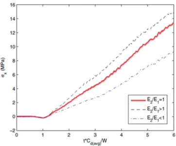
A detailed stress history analysis is performed to obtain the influence of material gradation on the bending behavior of the beam.Figure 3shows the bending stress (σx) history of point P due to impact velocity of 5 m/s for the three cases mentioned above with normalized time t⁰= t*Cd/W as the x-axis and stress (MPa) as the y-axis.

We see that material gradation leads to considerable change in the stress field at point P. The stress wave takes normalized time of about 0.7 to reach the point P, which is different from 0.8 in Zhang and Paulino [42]. This is due to 3D effects. In a 3D medium, stress waves travel at different speeds when compared to a 2D

medium. At this time, the point P undergoes compressive stress until the

Figure 2.

Epoxy/glass beam subjected to velocity impact: (a) geometry and boundary conditions of the three-point bending specimen and (b) one-quarter model with symmetric boundary conditions. Stress values are retrieved at P(0, 0.2 W). (c) 3D FE mesh of the one-quarter model. The FE mesh contains 14,085 15-node wedge elements and 44,827 nodes. (d) Zoom of the FE mesh near the left bottom corner, i.e., at x = 0.

(37)

normalized time of around 1.1. This compressive stress is due to the Poisson’s ratio (ν) effect. In a separate simulation of the beam under similar loading conditions, the Poisson’s ratio of the beam was made zero, and we found that the point P

underwent tensile stress throughout the simulation (result not shown). From this instant, i.e., after normalized time of 1.1, the point P undergoes monotonically increasing tensile stress. The maximum tensile stress is consistently attained in the StiffTop beam, and the minimum in the StiffBot beam and the Homog beam undergoes stresses in between these two. This type of behavior may be intuitively observed as the material properties (E,ρ) of a StiffTop beam at point P are lower than the StiffBot and Homog beams and hence may undergo higher stresses. We also found that for the line load, the stress componentσxalong the thickness (z) direction at point P(y = 0.2 W) does not vary considerably.

Figure 4shows the stress history of componentσyat point P for different material gradations due to impact velocity of 5 m/s. We see that there is a considerable effect of the gradation on this stress behavior, too. The first stress wave approaches point P at normalized time of 0.7 due to the compressive velocity loading. At this point, there is a sudden increase inσystress magnitude (compressive) until a normalized time of 1.25. The stress wave reaches the bottom surface of the beam and reflects as tensile waves at which point there is a gradual decrease in the compressive stress until the normalized time of 2.0. Between normalized times 2.0 and 2.7, the stress behavior does not change considerably, although there are small variations, which may be because of the discrete wave reflections from the edges that occur in finite configurations, to form a plateau in the stress field. The stress wave, after reflecting from the top surface, becomes compressive and leads to an increase in compressive stress between normalized times 2.7 and 3.2. Between the normalized times of 3.2 and 6, the stress behavior tends to repeat itself as seen between 0.7 and 3.2, although with larger variations of increase and decrease. The results plotted inFigures 13and14are consistent with the plane stress simulation results obtained by Zhang and Paulino [42] and Rousseau and Tippur [38].

Figure 5shows the 2D contour plot of the stress componentσxat a specific time instant of 90μs (t⁰�5.9) for the three beams subjected to the impact velocity of 5 m/s. We firstly see that the stress pattern is considerably different among the

Figure 3.

Stress historyσ_xat location P (0, 0.2 W) for homogeneous and graded beams with linearly varying E andρ, subjected to velocity impact (V = 5 m/s) at the top.