The formulations of the theories of special and general relativity and of the theory of quantum mechanics in the first decades of the twentieth century are a fundamental milestone in science, because of their profound implications not only for physics, but also for research methodology. In this textbook, the theories of special and general relativity are introduced using the Lagrangian formalism.
Special Principle of Relativity
Although it is possible to describe physical phenomena even in non-inertial frames of reference, namely in the frames of reference that do not belong to the class of inertial frames of reference, the description is more complicated. With the concept of inertial frame of reference, we can introduce the special principle of relativity.
Euclidean Space
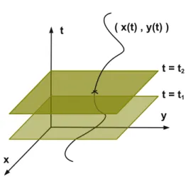
It is straightforward to apply Eq. 1.11) and see that in spherical coordinates the square of the line element is. The length of a curve between two points in space is also invariant.
Scalars, Vectors, and Tensors
For example, if we have the tensor Aab and lower the subscripts, we should write Aab. If we have a tensor of type (r,s) and order r+s and shrink 2t indices, the new tensor is of type (r−t,s−t) and order r+s−2t.
Galilean Transformations
8 1 Introduction If we increase an index of the metric tensor, we get the Kronecker delta,gi jgj m =gim= δim. The rotations about the x, y, andzaxes (or, equivalently, the rotations in their z, x z, and x y planes) of the angle θ respectively have the following form.
Principle of Least Action
If we require that the operation of Si is stationary for every small variation of the Lagrangian coordinates of the system, i.e. δS=0 for any δqi, we get the Euler–Lagrange equations. In such a case, the Lagrangian of the system is simply given by the difference between the point particle's kinetic energy T and its potential V .
Constants of Motion
Equation (1.55) is the well-known Newton's second law for a point-like particle in a potential V, and therefore the Lagrangian in Eq. Since V = 0, the Lagrangian of the system is just the kinetic energy of the particle.
Geodesic Equations
Note that the geodesic equations can be obtained even if we apply the principle of least action to the length of the particle's trajectory. Of course, the choice of the parameterization does not affect the solution of the equations.
Newton ’ s Gravity
If the motion of the particle is initially in the equatorial plane, namely θ(t0)=π/2 and θ(t˙ 0)=0, where is an initial time, it remains in the equatorial plane. 5We use the notation Lz because this is the axial component of angular momentum and we don't want to call it L because it can cause confusion with the Lagrangian.
Kepler ’ s Laws
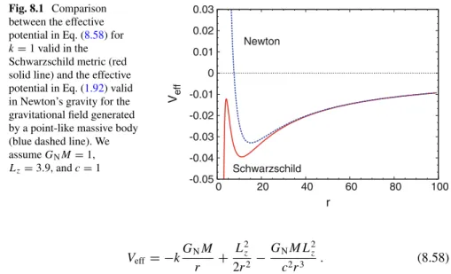
The first term on the right-hand side in (1.92) is the (attractive) gravitational potential of a point body of mass M and dominates when the particle is at large radii. The solutions of the differential equations in (1.100) and (1.101) are the equations of a circle and a cone, respectively. 1.93), we can write the surface of the ellipse described by the planet's orbit as
Maxwell ’ s Equations
At the end of the 19th century, it was obvious to postulate the existence of a medium for the propagation of electromagnetic phenomena. At this point it was necessary to find direct or indirect evidence for the existence of the aether.
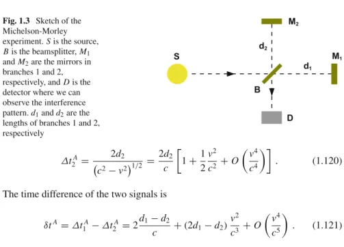
Michelson – Morley Experiment
Considering the velocity of the Solar System around the galactic center, which is about 220 km/s, we should expect δn=3. Strictly speaking, these experiments do not rule out the hypothesis of the existence of the ether if we postulate space.
Towards the Theory of Special Relativity
Write the Lagrangian in cylindrical coordinates and then the corresponding Euler–Lagrange equations. It is the Lagrangian of a particle moving in 2-dimensional space and subject to a potential V =k(x2+y2)/2.
Einstein ’ s Principle of Relativity
The electromagnetic signal simultaneously reaches all points equidistant from the origin. Now let's look at the reference frame (x,y,z) moving with velocity v relative to the reference frame (x,y,z).
Minkowski Spacetime
In Newtonian mechanics, if the rate of propagation of interactions was finite, its value must change in different frames of reference. If we measure the velocity in the (x,y,z) reference frame, in the (x,y,z) reference frame, moving at constant speed relative to the (x,y,z) reference frame, the velocity of propagation of the interaction must be bew=w−vand can exceed the speed of light in a vacuum.
Lorentz Transformations
The generalization of the Galilean transformations should therefore come from the rotations in the plane x,˜t y,˜ ent z.˜. Note that d x/dt= −v, where−vis is the velocity of the reference frame(ct,x,y,z) relative to the reference frame(ct,x,y,z), and thus.
Proper Time
The twins from the spacecraft will now be younger than the twins who stayed on Earth. The twin of the spacecraft is not in an inertial reference frame, because otherwise he/she could not return to Earth.
Transformation Rules
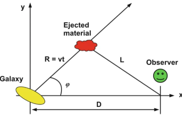
Superluminal Motion
Given this RD, we can calculate the distance L between the position of the ejected material in time and the observer. The apparent velocity of the ejected material along the yaxis measured by a distant observer is.
Example: Cosmic Ray Muons
In the rest frame of the muon, the time the particle takes to reach the surface of the Earth is Δt=Δt/γ ≈5µs. In the rest frame of the muon, the Earth moves at velocity v=0.995c and has Lorentz factor γ =10.
Action for a Free Particle
However, in general it is not convenient to parameterize the particle trajectory with the coordinate time, i.e. xμ=xμ(t). With a signed metric (+ − −−), as is the common convention among the particle physics community, we can write Eq.
Momentum and Energy
The energy of the particle (Hamiltonian) is obtained from the Legendre transform of the Lagrangian. The conjugate momentum of the particle is pμ= ∂L. 3.5), we have the conservation of the particle mass.
Massless Particles
Such an additional term can always be removed by a suitable reparameterization, which is the case when we use an affine parameter.
Particle Collisions
Let us now consider the frame of reference in which the total 3-momentum of the system vanishes, namely pi=pf =0.
Example: Colliders Versus Fixed-Target Accelerators
Now is the 4 momenta of the two particles (assuming the positron moves along the x-axis). m2ec4+p2c2is now just the energy of the positron. 3.56). With a fixed-target experiment, we would have to accelerate one of the two particles to 8000 TeV to get the same reaction.
Example: The GZK Cut-Off
Now let's assume that we want the same reaction in a fixed-target accelerator, namely we accelerate the positron and we fire it against an electron that is at rest in the reference frame of the laboratory. Protons with energies above 1020eV interact with the CMB photons and lose energy, so they cannot travel long distances in the Universe.
Multi-body Systems
The total energy of the system seen as a single body and as a connected state consisting of a number of more elementary components must be the same. The total energy of the bound state includes the rest energy of the single components, their kinetic energies, and all interaction terms.
Lagrangian Formalism for Fields
For example, in the case of a free point particle moving in 3-dimensional space in Newtonian mechanics, the Lagrangian is the kinetic energy of the particle, and the Lagrangian coordinates can be the Cartesian coordinates of the particle. If we go from Cartesian coordinates to non-Cartesian coordinates, we need to calculate the determinant of the Jacobian, J and d3V.
Energy-Momentum Tensor
If we change the sign in Eq. 3.88), then Ttti is minus the energy density of the system [see later after Eq. T0is are thus the three components of the energy flux density. Ti js can be interpreted as the components of the momentum flux density.
Examples
Energy-Momentum Tensor of a Free Point-Like
Ti js are proportional to the components of the momentum flux density and therefore we need to add one more velocity. Finally we have the following expression for the energy-momentum tensor of a free particle as a point in Cartesian coordinates.
Energy-Momentum Tensor of a Perfect Fluid
Calculate the threshold energy of the high-energy photon that allows the reaction.me+c2 =me−c2=0.5 MeV. The electric field can therefore be written in terms of the scalar potentialφ and the vector potentialA.
Action
The electric and magnetic fields can be written in terms of the Faraday tensor as follows. The space-time components of the Faraday tensor can be written in terms of the magnetic field.
Motion of a Charged Particle
Now let's parameterize the trajectory of the particle with the proper time τ of the particle. where τ is the proper time of the particle, the Lagrangian terms are Lm = 1. and now the dot˙denotes the derivative of toτ, i.e. x˙μ=d xμ/dτ. If we do not use Cartesian coordinates, in Eq. 4.36) we have gμν instead ofημν, Lm gives the geodesic equations, and Eq.
Maxwell ’ s Equations in Covariant Form
Homogeneous Maxwell ’ s Equations
Using the relations in (4.16), we replace the Faraday tensor components with electric and magnetic field components.
Inhomogeneous Maxwell ’ s Equations
Since Fμν is antisymmetric tensor, ∂ν∂μFμν=0, and thus we find conservation of electric current. If there is no output/input of electric current, we have storage of electric charge in that region.
Gauge Invariance
Thus, equation (4.62) tells us that any change in the total electric charge can be accounted for by the output/input of the electric current at the boundary of the region.
Energy-Momentum Tensor of the Electromagnetic Field
We will see in Sect.7.4 that it is possible to define the energy moment tensor without ambiguities. Finally, it is worth noting that the energy-momentum tensor of the electromagnetic field has a vanishing trace.
Examples
Motion of a Charged Particle in a Constant Uniform
Thus, the energy of the particle is (here we use ε to denote the energy of the particle because E is the electric field). In relativistic theory, the speed of charged particles asymptotically approaches the speed of light.
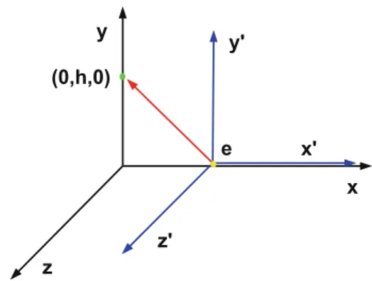
Electromagnetic Field Generated by a Charged
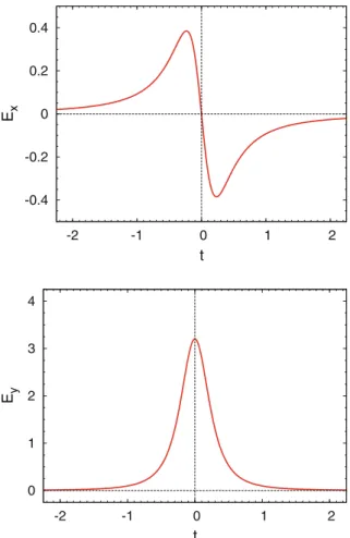
In the reference frame with the Cartesian coordinates (x,y,z), the particle is at rest at the point x=(0,0,0). The x-component of the electric field in the reference frame (x,y,z) at the point x=(0,h,0) is shown in fig. 4.2 as a function of time.
Motivations
In contrast, the ratio of inertial to gravitational mass, mi/mg, is a constant independent of the particle. Thus, we can choose units in which mi=mg =m, where only the mass of the particle is.
Covariant Derivative
De fi nition
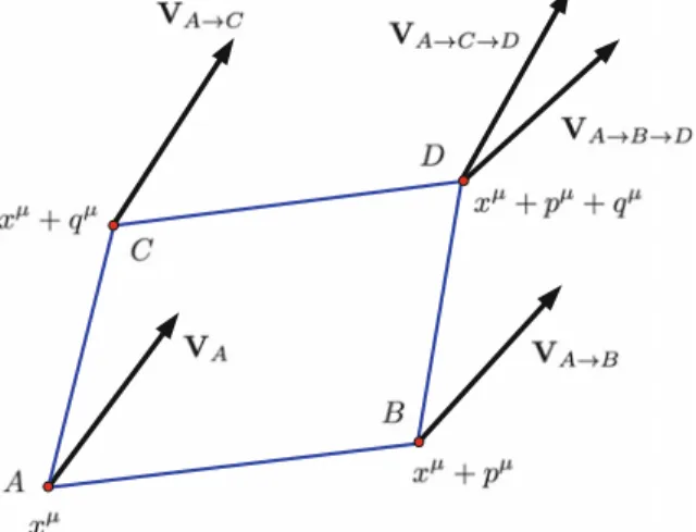
Parallel Transport
Intuitively, you should "transfer" one of the two vectors to a point of the other vector and calculate the difference there. Now we want to see that the coordinates of the atBar vector are given by . 5.41).
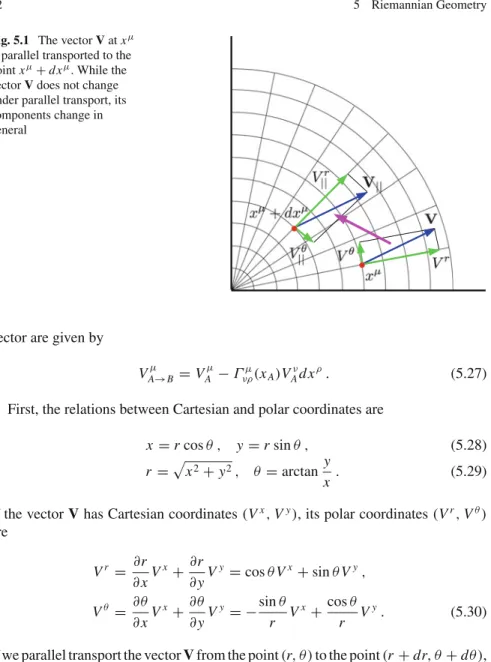
Properties of the Covariant Derivative
Note that the sign in front of the Christoffel symbols is now plus because we are transporting a vector from x+d x tox, while in Eq.
Useful Expressions
Using Eq. 5.63), the covariant divergence of a generic vector Aμ can be written as.
Riemann Tensor
- De fi nition
- Geometrical Interpretation
- Ricci Tensor and Scalar Curvature
- Bianchi Identities
We can now write the Riemann tensor Rλρνμ in terms of Christoffel symbols as follows. 5.71). Rμνρσ+Rμρσ ν+Rμσ νρ and can be easily verified using the explicit expression of the Riemann tensor in Eq.
General Covariance
An alternative formulation of the idea that the laws of physics are independent of the choice of frame of reference is the principle of general covariance. General relativity allows us to deal with non-inertial reference frames and phenomena in gravitational fields.
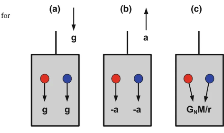
Einstein Equivalence Principle
The local positional invariance requires the non-gravity laws of physics to be the same at all points of spacetime; for example, this prohibits variation of fundamental constants. In local free-falling frames of reference, the non-gravity laws of physics are the same as in special relativity.
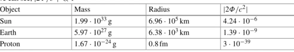
Connection to the Newtonian Potential
The theories of gravity that satisfy Einstein's equivalence principle are the so-called metric theories of gravity, which are defined as follows: Table 6.1 shows the value of |2Φ/c2| on their surface for the Sun, the Earth, and the proton.
Locally Inertial Frames
Locally Minkowski Reference Frames
Locally Inertial Reference Frames
The motion of a test particle around the origin in this reference frame is the same as in special relativity in Cartesian coordinates and we can therefore say that we have locally removed the gravitational field.
Measurements of Time Intervals
In this particular example, the temporal coordinate coincides with the proper time τ forr → ∞, which means that the reference frame corresponds to an observer's coordinate system at infinity. In general, Δτ < Δt, and the observer's clock in the gravitational field is slower than an observer's clock at infinity.
Example: GPS Satellites
Δt, and the clock of an observer in the gravitational field is slower than the clock of an observer at infinity. For GPS satellites, the distance from the center of the Earth is r=26600 km. 6.35), we can write the relation between the appropriate time interval of the GPS receiver Δτ and the appropriate time interval of the GPS satellites Δτ.
Non-gravitational Phenomena in Curved Spacetimes
For now, there are no experiments that can test the presence of the term ξRφ2, in the sense that it is only possible to limit the parameter ξ below a huge unnatural value. General covariance is the basic principle: once we have the metric of spacetime, we can describe non-gravitational phenomena.
Einstein Equations
Finally, note that the Einstein equations relate the geometry of spacetime (on the left) to the matter content (on the right). In principle, we can obtain any kind of spacetime for proper choice of the matter-energy momentum tensor.
Newtonian Limit
In other words, Einstein's equations can make clear predictions only if we clearly determine the content of matter. After replacing Rtt with ΔΦ/c2 in equation 7.17) with Poisson's equation ΔΦ=4πGNρ, valid in Newton's theory, we find the relationship between κinGN.
Einstein – Hilbert Action
The natural candidates for the Lagrangian coordinates of the action of the gravitational field are the metric coefficients and their first derivatives, namely gμν and . Finally, we need to calculate the effect of a variation of the metric coefficients on the Ricci tensor.
Matter Energy-Momentum Tensor
De fi nition
Examples
When we consider the variation of the metric tensor, we find that δS= 1. 7.54) and is therefore the energy and momentum tensor of a free point particle. 7.55). The operation of a real scalar field in curved spacetime is S= −. When we consider the variation of the metric coefficients, we find δS = −. 7.59).
Covariant Conservation of the Matter
Pseudo-Tensor of Landau – Lifshitz
Analytical solutions to Einstein's equations can be found when spacetime has certain special symmetries. The Schwarzschild metric is a relevant example of an exact solution of Einstein's equations with important physical applications.
Spherically Symmetric Spacetimes
The Einstein equations (7.6) relate the geometry of spacetime, encoded in the Einstein tensorGμν, to the matter content, described by the matter's energy-momentum tensorTμν. If we assume to be in Einstein's gravity, we can solve the Einstein equations with the approach in (8.8) to find the explicit form of the functions f andgin Einstein's gravity for a certain matter distribution.
Birkhoff ’ s Theorem
Comparing the geodesic equations with the last expression in (8.12), we see that the only non-vanishing Christoffel symbols are of the type Γμνt. Eventually, the line element of spacetime can be written in the following form. indicating that the metric is independent of.
Schwarzschild Metric
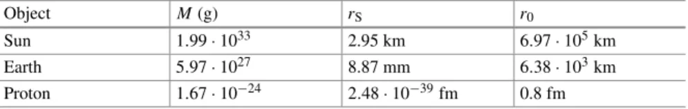
As can be seen in Appendix F, M can only be associated with the true mass of the body in the Newtonian limit. The relationship between the temporal coordinate of the Schwarzschild metric,t, and the proper time of an observer at a point with fixed(r, θ, φ)is.
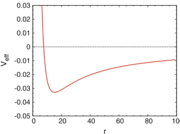
Motion in the Schwarzschild Metric
The effective potential Veff in Eq. 8.58) can be compared with the Newtonian effective potential in Eq. Fork=1, we see that the first and second terms on the right-hand side in Eq. The equations of the trajectories are thus. 8.64), we find circular orbits as in the Newtonian case from Eq.
Schwarzschild Black Holes
The singularity of the metric atr=rS depends on the choice of the coordinate system and can be removed by a coordinate transformation.4 For example, the Lemaitre coordinates(cT,R, θ, φ) are defined as. The maximum analytic extension of Schwarzschild spacetime is found when we use the Kruskal-Szekeres coordinates.
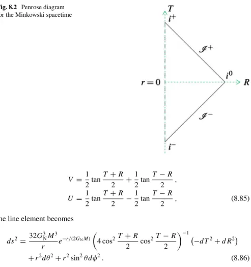
Penrose Diagrams
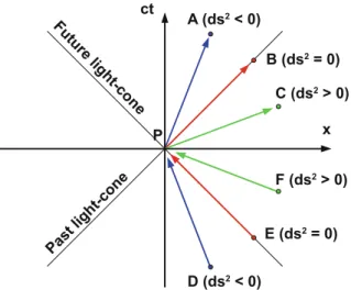
Minkowski Spacetime
The Schwarzschild solution in Kruskal–Szekeres coordinates also includes a white hole and a parallel universe, which are not present in Schwarzschild spacetime in Schwarzschild coordinates.
Schwarzschild Spacetime
Figure 8.3 shows the Penrose diagram for the maximum extension of Schwarzschild spacetime with its asymptotic regions i+,i−,i0,I+ and I−. Show the trajectories of the massive particle and of the electromagnetic pulse in the Penrose diagram.
Gravitational Redshift of Light
Equation (1.101) has the solution (1.103) and the trajectories are ellipses, parabolas or hyperbolas according to the value of the constant A. Equation (9.2) has the last term proportional tou2, which is absent in Newtonian gravity and introduces relativistic corrections. 9.9) Equation (9.9) shows that, as measured in the coordinate system (ct,r, θ, φ), the time intervals of the electromagnetic signal at the location of the observer and the observer are the same.
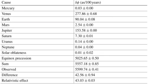
Perihelion Precession of Mercury
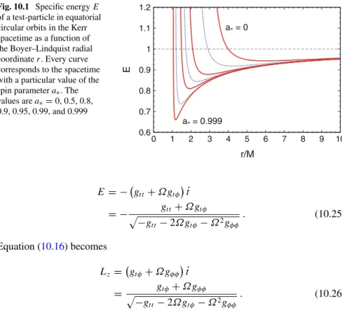
Time-like circular orbits in the equatorial plane of the Kerr metric are especially important [4]. First we find the radius of the marginally bounded circular orbit, defined by the condition E =1.
De fl ection of Light
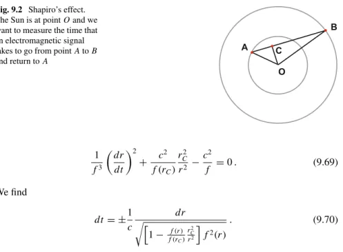
Shapiro ’ s Effect
In 1964, Irwin Shapiro proposed a new test, often called the fourth classical test of general relativity, which is based on measuring the time delay of an electromagnetic signal to travel from one point to another in the solar system relative to the time that it same signal would take in a flat spacetime [4]. To get an idea of the size of the effect, let's estimate the time delay of an electromagnetic signal to go from Earth to Mercury and return to Earth when the two planets are on opposite sides of the Sun, sorC is the Sun's radius.
Parametrized Post-Newtonian Formalism
The mass of the black hole M sets the size of the system and the corresponding length and time scales are, respectively. Note that the topology of the spacetime singularity in the Kerr solution is different from those in the Schwarzschild and Reissner–Nordström spacetimes.
De fi nition
Reissner – Nordstr ö m Black Holes
In Einstein's gravity, the simplest black hole solution is represented by the Schwarzschild spacetime described in ch. For the black hole solutions discussed in this textbook (Schwarzschild, Reissner–Nordström, Kerr), the radial coordinate of the event horizon corresponds to the larger root vangrr =0.
Kerr Black Holes
Equatorial Circular Orbits
Moreover, the minimum of the energy E and of the axial component of the angular momentum is located at the same radius. Figure 10.3 shows the radius of the event horizonr+, of the photon orbitrγ, of the marginally bound circular orbitrmb, and of the inner stable circular orbitrISCO in the Kerr metric in Boyer–Lindquist coordinates as functions of a∗.
Fundamental Frequencies
Frame Dragging
No-Hair Theorem
Gravitational Collapse
Dust Collapse
Homogeneous Dust Collapse
Penrose Diagrams
Reissner – Nordstr ö m Spacetime
Kerr Spacetime
Oppenheimer – Snyder Spacetime
Friedmann – Robertson – Walker Metric
Friedmann Equations
Cosmological Models
Einstein Universe
Matter Dominated Universe
Radiation Dominated Universe
Vacuum Dominated Universe
Properties of the Friedmann – Robertson – Walker Metric
Cosmological Redshift
Particle Horizon
Primordial Plasma
Age of the Universe
Destiny of the Universe
Historical Overview
Gravitational Waves in Linearized Gravity
Harmonic Gauge
Transverse-Traceless Gauge
Quadrupole Formula
Energy of Gravitational Waves
Examples
Gravitational Waves from a Rotating Neutron Star
Gravitational Waves from a Binary System
Astrophysical Sources
Coalescing Black Holes
Extreme-Mass Ratio Inspirals
Neutron Stars
Gravitational Wave Detectors
Resonant Detectors
Interferometers
Pulsar Timing Arrays
Spacetime Singularities
Quantization of Einstein ’ s Gravity
Black Hole Thermodynamics and Information Paradox
Cosmological Constant Problem
Suggestions for Solving the Problems