An Effective and Efficient Approach to Classification with Incomplete Data
Cao Truong Trana,b,∗, Mengjie Zhanga, Peter Andreaea, Bing Xuea, Lam Thu Buib
aSchool of Engineering and Computer Science, Victoria University of Wellington, PO Box 600, Wellington 6140, New Zealand
bResearch Group of Computational Intelligence, Le Quy Don Technical University, 236 Hoang Quoc Viet St, Hanoi, Vietnam.
Abstract
Many real-world datasets suffer from the unavoidable issue of missing values.
Classification with incomplete data has to be carefully handled because inad- equate treatment of missing values will cause large classification errors. Us- ing imputation to transform incomplete data into complete data is a common approach to classification with incomplete data. However, simple imputation methods are often not accurate, and powerful imputation methods are usually computationally intensive. A recent approach to handling incomplete data con- structs an ensemble of classifiers, each tailored to a known pattern of missing data. The main advantage of this approach is that it can classify new incomplete instances without requiring any imputation. This paper proposes an improve- ment on the ensemble approach by integrating imputation and genetic-based feature selection. The imputation creates higher quality training data. The feature selection reduces the number of missing patterns which increases the speed of classification, and greatly increases the fraction of new instances that can be classified by the ensemble. The results of experiments show that the proposed method is more accurate, and faster than previous common methods for classification with incomplete data.
Keywords: incomplete data, missing data, classification, imputation, feature
∗Corresponding author. Tel: +64221587242
Email address: [email protected](Cao Truong Tran )
selection, ensemble learning
1. Introduction
Classification is one of the most important tasks in machine learning and data mining [1]. Classification consists of two main processes: a training process and an application (test) process, where the training process builds a classifier which is then used to classify unseen instances in the application process. Clas-
5
sification has been successfully applied to many scientific domains such as face recognition, fingerprint, medical diagnosis and credit card fraud transaction.
Many algorithms have been proposed to deal with classification problems, but the majority of them require complete data and cannot be directly applied to data with missing values. Even when some methods can be applied, missing
10
values often lead to big classification error rates due to inadequate information for the training and application processes [2].
Unfortunately, missing values are a common issue in numerous real-world datasets. For example, 45% of the datasets in the UCI machine learning repos- itory [3], which is one of the most popular benchmark databases for machine
15
learning, contain missing values [2]. In an industrial experiment, results can be missing due to machine failure during the data collection process. Data collected from social surveys is often incomplete since respondents frequently ignore some questions. Medical datasets usually suffer from missing values because typically not all tests can be done for all patients [4, 5]. Financial datasets also often
20
contain missing values due to data change [6, 7].
One of the most common approaches to classification with incomplete data is to use imputation methods to substitute missing values with plausible values [4, 8, 9]. For example, mean imputation replaces all missing values in a feature by the average of existing values in the same feature. Imputation can provide
25
complete data which can then be used by any classification algorithm. Simple imputation methods such as mean imputation are often efficient but they are often not accurate enough. In contrast, powerful imputation methods such as
multiple imputation [10] are usually more accurate, but are computationally expensive [11, 12]. It is not straightforward to determine how to combine classi-
30
fication algorithms and imputation in a way that is both effective and efficient, particularly in the application process.
Ensemble learning is the process of constructing a set of classifiers instead of a single classifier for a classification task, and it has been proven to improve classification accuracy [13]. Ensemble learning also has been applied to clas-
35
sification with incomplete data by building multiple classifiers in the training process and then applicable classifiers are selected to classify each incomplete instance in the application process without requiring any imputation method [14, 15, 16]. However, existing ensemble methods for classification with incom- plete data often cannot work well on datasets with numerous missing values
40
[14, 16]. Moreover, they usually have to build a large number of classifiers, which then require a lot of time to find applicable classifiers for each incomplete instance in the application process, especially when incomplete datasets contain a high proportion of missing values [14, 15]. Therefore, how to construct a com- pact set of classifiers able to work well even on datasets with numerous missing
45
values should be investigated.
Feature selection is the process of selecting relevant features from original fea- tures, and it has been widely used to improve classification with complete data [17]. Feature selection has also been investigated in incomplete data [18, 19], but the existing methods typically still use imputation to estimate missing val-
50
ues in incomplete instances before classifying them. By removing redundant and irrelevant features, feature selection has the potential of reducing the num- ber of incomplete instances, which could then improve accuracy and speed up classifying incomplete instances. However, this aspect of feature selection has not been investigated. This paper will show how to utilise feature selection to
55
improve accuracy and speed up the application process for classification with incomplete data.
1.1. Goals
To deal with the issues stated above, this paper aims to develop an effec- tive and efficient approach for classification with incomplete data, which uses
60
three powerful techniques: imputation, feature selection and ensemble learning.
Imputation is used to transform incomplete training data to complete train- ing data which is then further enhanced by feature selection. After that, the proposed method builds a set of specialised classifiers which can classify new incomplete instances without the need of imputation. The proposed method
65
is compared with other common approaches for classification with incomplete data to investigate the following main objectives:
1. How to effectively and efficiently use imputation for classification with incomplete data; and
2. How to use feature selection for classification with incomplete data to
70
not only improve classification accuracy but also speed up classifying new instances; and
3. How to build a set of classifiers which can effectively and efficiently classify incomplete instances without the need of imputation; and
4. Whether the proposed method can be more accurate and faster than using
75
imputation both in the training process and the application process; and 5. Whether the proposed method can be more accurate and faster than the
existing ensemble methods.
1.2. Organisation
The rest of this paper is organised as follows. Section 2 presents a survey of
80
related work. The proposed method is described in Section 3. Section 4 explains experiment design. The results and analysis are presented and discussed in Section 5. Section 6 states conclusions and future work.
2. Related Work
This section firstly introduces traditional approaches to classification with
85
incomplete data. It then discusses ensemble learning for classification with
incomplete data. Finally, it presents typical work on feature selection.
2.1. Traditional Approaches to Classification with Incomplete Data
There are several traditional approaches to classification with incomplete data. The deletion approach simply deletes all instances containing missing
90
values. This approach is limited to datasets with only a few missing values in the training data and no missing values in the application process [20]. A second approach is to use one of classifies such as C4.5 which can directly classify incomplete datasets using a probabilistic approach [21]. However, their accuracy is limited when there are a lot of missing values [22].
95
The most used approach to classification with incomplete data is to use imputation methods to transform incomplete data into complete data before building a classifier in the training process or classifying a new incomplete in- stance in the application process. This approach has the advantage that the imputed complete data can be used by any classification algorithm. This ap-
100
proach also can deal with incomplete datasets with a large number of missing values [8, 23].
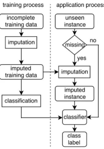
Fig. 1 shows the main steps using imputation for classification with incom- plete data. In the training process, imputation is used to estimate missing values for incomplete training data. After that, imputed training data is put into a
105
classification algorithm to build a classifier. In the application process, complete instances are directly classified by the classifier. With each incomplete instance, its missing values are first replaced by plausible values by using the imputation to generate a complete instance which is then classified by the classifier.
There are two classes of imputation: single imputation and multiple impu-
110
tation.
2.1.1. Single Imputation
Single imputation estimates a single value for each missing value. Mean imputation is an example of single imputation methods which fills all missing values in each feature by the average of all existing values in the same feature.
115
Figure 1: A common approach to using imputation for classification with incomplete data.
kNN-based imputation is one of the most powerful single imputation meth- ods [22]. To estimate missing values in an incomplete instance, it first searches for itsknearest neighbour instances. After that, it replaces missing values of the instance with the average of existing values in thekinstances. kNN-based impu- tation is often more accurate than mean imputation [22]. However, kNN-based
120
imputation is more computationally expensive than mean imputation because it takes time to find the nearest instances, especially with datasets containing a large number of instances and a large value ofk [22].
Single imputation has been widely used to estimate missing values for clas- sification with incomplete data [8, 20, 23, 22]. In [20] and [22], kNN-based
125
imputation is shown to outperform C4.5, mean imputation and mode imputa- tion. In [23], the impact of six imputation methods on classification accuracy for six classification algorithms are investigated. Results show imputation on average can improve classification accuracy when compared to without using imputation. However, in [8], fourteen different imputation methods are evalu-
130
ated on three different classification algorithm groups. The analysis shows that there is no best imputation for all classifiers.
2.1.2. Multiple Imputation
Multiple imputation estimates a set of values for each missing value. Multiple imputation is often better than single imputation because it can better reflect
135
the uncertainty of missing data than single imputation [11]. However, multiple imputation is usually more computationally expensive than single imputation since it takes time to estimate a set of values for each missing value [4].
Multiple imputation using chained equations (MICE) is one of the most flex- ible and powerful multiple imputation methods [10, 24]. MICE uses regression
140
methods to estimate missing values. Initially, each missing value in each feature is replaced by a random value in the same feature. Each incomplete feature is then regressed on the other features to compute a better estimate for the feature. The process is performed several times (q) for all incomplete features to provide a single imputed dataset. The whole procedure is repeatedptimes
145
to providepimputed datasets. Finally, the final imputed dataset is calculated by the average of thep imputed datasets [10, 24].
Multiple imputation has also been applied to classification with incomplete data [11, 12, 25]. In [11], multiple imputation methods are compared with single imputation methods. The study shows that multiple imputation methods are
150
often more accurate, but more expensive than single imputation methods. In [25], MICE is compared to other four single imputation methods. Results show that MICE can outperform the other single imputation methods, especially on datasets containing numerous missing values. In [12], ensemble learning is combined with multiple imputation to construct a set of classifiers. Each
155
imputed dataset which is generated by the multiple imputation method is used to build a classifier. The analysis shows that the proposed method can normally obtain better accuracy than using multiple imputation.
Existing imputation researches for classification often focus on improving classification accuracy [22, 25]. However, using imputation takes time to esti-
160
mate missing values, especially powerful imputation such as MICE is computa- tionally intensive. Therefore, how to effectively and efficiently use imputation
for classification should be further investigated.
2.2. Ensemble Classifiers for Incomplete Data
Ensemble learning is a learning method which constructs a set of base clas-
165
sifiers for a classification task in the training process. To classify new instances in the application process, the predictions of base classifiers are combined. En- sembles of classifiers have been proven to be more accurate than any of base classifiers making up the ensemble [13].
Ensemble learning also has been used for classification with incomplete data.
170
One of the first work using ensembles for classification with incomplete data ap- pears in [26], where four neural networks are built to address classification with a thyroid disease database consisting of two incomplete features (one classifier that ignores both the missing features, two classifiers that can be used if one of the features is present, and one classifier that requires both features to be
175
present). Experimental results show that the ensemble is superior to an impu- tation method using neural networks to estimate missing values. The ensemble is also more accurate than an induction algorithm which builds a decision tree able to directly work with incomplete data. The systems described in [14] and [27] tackle incomplete data by learning a set of neural networks, where each neu-
180
ral network is trained on one complete sub dataset extracted from incomplete data by dropping some of missing features. Given a new incomplete instance to classify, the available learnt classifiers are combined to classify the instance without requiring imputation. Empirical results show that the ensembles of neural networks can achieve better accuracy than two other ensemble methods
185
(based on bagging and boosting) combined with mean and mode imputations.
A similar approach is proposed in [28], where conditional entropy is used as the weighting parameter to reflect the quality of feature subsets which are used to build base classifiers. The proposal of [28] is extended in [16] by using the mutual information criterion to eliminate redundant feature subsets. As a re-
190
sult, the extended system can not only outperform other methods, but can also reduce the computation time to classify incomplete instances. In [15] and [29],
an ensemble of numerous classifiers is constructed, where each base classifier is trained on a sub dataset by randomly selecting a feature subset from the original features. Thanks to constructing a larger number of base classifiers, the system
195
can cope with incomplete data containing a high proportion of missing values.
Existing ensemble methods for classification with incomplete data can deal with missing values to some extent. However, the ensemble methods usually do not obtain good accuracy when datasets contain a large number of missing values [14, 16, 26]. The underlying reason is that the complete sub datasets
200
often only have a small number of instances when the original incomplete data includes a large number of missing values. Therefore, the base classifiers trained on the complete sub datasets are weak classifiers. To overcome the problem, numerous base classifiers have to be built [15], which requires a long time for exploring available classifiers to classify new incomplete instances. Therefore,
205
how to build an effective and efficient ensemble for classification with datasets containing numerous missing values should be further investigated.
2.3. Feature Selection for Classification
The purpose of feature selection is to select a subset of relevant features from the original features because many datasets often contain irrelevant and/or
210
redundant features which can be removed without losing much information. By removing irrelevant and redundant features, feature selection can reduce the training time, simplify the classifier and improve the classification accuracy [17]. However, feature selection is a hard problem because there are 2n possible feature subsets wherenis the number of original features [30].
215
A feature selection method consists of two main components: an evaluation measure and a search technique [17]. The evaluation measure is used to evaluate the goodness of selected features while the search technique is used to explore new feature subsets. The quality of the feature selection method strongly de- pends on both the evaluation measure and the search technique [17, 30].
220
Evaluation measures for feature selection can be divided into wrapper meth- ods and filter methods [17]. A wrapper method employs a classification algo-
rithm to score feature subsets while a filter method employs a proxy measure such as mutual information to score feature subsets. Filter methods are often more efficient and general than wrapper methods. However, wrapper meth-
225
ods tend to more accurate than many filter methods because wrapper methods directly evaluate feature subsets using classification algorithms while filter meth- ods are independent of any classification algorithm [17].
Search techniques for feature selection can be categorised into deterministic search techniques and evolutionary search techniques [17]. Sequential forward
230
selection (SFS) and sequential backward selection (SBS) are typical examples of deterministic search techniques [31]. In recent years, Evolutionary Computation (EC) techniques such as Genetic Algorithms (GAs), Genetic Programming(GP) and Particle Swarm Optimisation (PSO) have been successfully applied to fea- ture selection [17]. The underlying reason is that EC techniques are good at
235
searching for global best solutions. EC techniques also do not require domain knowledge and do not require any assumption related to the search space [17].
Feature selection has also been used for incomplete data [18, 32, 19]. How- ever, these methods still provide incomplete data which cannot be directly used by the majority of classification algorithms. Therefore, how to apply feature se-
240
lection to improve the performance of such classification algorithms when facing with missing values should be investigated.
3. The Proposed Method
This section presents the proposed method in detail. It starts with showing the definitions used in the method. The section then presents the overall struc-
245
ture and the underlying ideas of the method. After that, it describes the details of the training process and the application process.
3.1. Definitions
LetD={(Xi, ci)|i= 1, .., m}denote a dataset, where eachXirepresents an input instance with its associated class labelci, andmis the number of instances
250
in the dataset. The input space is defined by a set ofnfeaturesF ={F1, ..., Fn}.
Each instanceXiis represented by a vector ofn values (xi1, xi2, ...xin), where an xij is either a valid value of thejthfeatureFj, or is the value “?”, which means that the value is unknown (a missing value).
An instance Xi is called an incomplete instance if it contains at least one
255
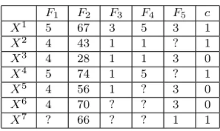
missing value. A dataset, D, is called an incomplete dataset if it contains at least one incomplete instance. A feature, Fj, is called an incomplete feature for a dataset if the dataset contains at least one incomplete instance,Xi with a missing value xij. For example, the incomplete dataset shown in Table 1 contains five incomplete instances: X2, X4, X5, X6, and X7. It has four
260
incomplete features: F1, F3,F4andF5.
Table 1: An example dataset with missing values.
F1 F2 F3 F4 F5 c
X1 5 67 3 5 3 1
X2 4 43 1 1 ? 1
X3 4 28 1 1 3 0
X4 5 74 1 5 ? 1
X5 4 56 1 ? 3 0
X6 4 70 ? ? 3 0
X7 ? 66 ? ? 1 1
A subset of features, S ⊂F, is called a missing pattern in a dataset D if there is at least one instance,XiinD, such that the value inXifor each feature inS is missing, and the value inXi for all the other features are known. That is,S⊂X is a missing pattern inDif there exists an instanceXiinD such that
265
ifFj ∈S, xij =? otherwise,xij is not missing. For example, the dataset shown in Table 1 has five missing patterns: {∅},{F5},{F4},{F3, F4}and{F1, F3, F4}.
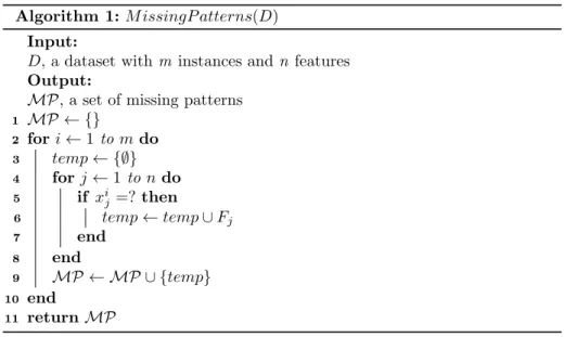
Algorithm 1 shows the steps to identify all missing patterns of a dataset. We useMP to denote the all missing patterns. At the beginning of the algorithm, MP is empty. The outer loop in the algorithm iterates over all instances. For
270
each instance, all features with missing values are combined to form a missing pattern. If the missing pattern is not yet inMP, it will be added inMP. By the end of the algorithm,MP contains all missing patterns.
Given a dataset D and a feature subset S, we use DS to represent the
Algorithm 1:M issingP atterns(D) Input:
D, a dataset withm instances andn features Output:
MP, a set of missing patterns
1 MP ← {}
2 fori←1 tomdo
3 temp← {∅}
4 forj←1 tondo
5 if xij =?then
6 temp←temp∪Fj
7 end
8 end
9 MP ← MP ∪ {temp}
10 end
11 returnMP
projected datasetD onto the features in S, i.e. the datasetD reduced to the
275
feature subset S. That is, each instance in D is replaced by the projected instance in which values for features not in S are removed. For example, given the dataset shown in Table 1 with five features, the data subsetD{F1,F2,F3} is shown in Table 2.
Table 2: The dataset in Table 1 reduced to the feature subset{F1, F2, F3}.
F1 F2 F3 c
X1 5 67 3 1
X2 4 43 1 1
X3 4 28 1 0
X4 5 74 1 1
X5 4 56 1 0
X6 4 70 ? 0
X7 ? 66 ? 1
3.2. Overall Proposed Method
280
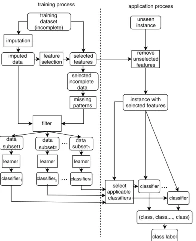
The proposed method has two main processes: a training process and an application process. The training process constructs an ensemble of classifiers which is then used to classify new instances in the application process. Fig. 2 shows the flowchart of the method.
The method is based on three key ideas. The first idea is that the method
285
Figure 2: The proposed method builds an ensemble of classifiers then used to classify new incomplete instances without imputation.
constructs an ensemble of classifiers to cover possible missing patterns, each classifier being built on one missing pattern. Therefore, new incomplete in- stances can be classified by the ensemble without requiring imputation. This is not a complete novel—it has also been used in [14, 16]. The second idea is to use imputation in the training process, but not in the application process. Using
290
a powerful imputation method to generate high quality complete training data for building classifiers results in more accurate classifiers. In contrast, existing ensemble methods based on missing patterns [14, 16] do not use any imputation, so the training set for each classifier may be as small as a single instances which leads to low accuracy. However, good imputation methods such as multiple
295
imputation are computationally expensive. For the training process, there is no time limit for many applications, and the high cost of multiple imputation is not a problem; in the application process, there may be tight time limits on the process of classifying a new instance, and using multiple imputation may be infeasible. The third idea is to use feature selection to further improve the
300
training data. By removing redundant and irrelevant features, feature selec- tion not only produces a high quality feature set, but also reduces the number of missing patterns and removes missing values of incomplete instances in the application process.
3.3. Training Process
305
The purpose of the training process is to build a set of classifiers, one classifier for each missing pattern in the data. Algorithm 2 shows the main steps of the training process. The inputs of the algorithm are an original training dataset Dand a classifier learning algorithmL.
Algorithm 2:The training process Input:
D, an original training dataset L, a classifier learning algorithm Output:
C, a set of learnt classifiers w, the weighting of classifiers SF, a set of selected features
1 ImpD←Imputation(D)
2 SF ←F eatureSelection(ImpD)
3 MP ←M issingP aterns(DSF)
4 C ← {}
5 foreachMPi ∈ MP do
6 CPi ← SF − MPi
7 DivideImpDCPi intoImpT rain andImpV alidation
8 classif ieri← L(ImpT rain)
9 C ← C ∪classif ieri
10 wi ←classif ieri(ImpV alidation)
11 end
12 returnC,wandSF ;
The algorithm starts by using an imputation method to estimate missing
310
values in the original dataset D to generate an imputed dataset ImpD which is complete. After that, a feature selection method is applied to the complete dataset ImpD to select the subset SF of important features which is then applied to the original training dataset to construct a projected (incomplete) dataset with just the features in SF. The missing patterns algorithm (Algo-
315
rithm 1) is then used to search for all missing patterns, MP, in the reduced datasetDSF. For each missing patternMPi, a “complete pattern”CPiis gen- erated by selecting features which are inSF, but not inMPi. After that, the imputed dataset is reduced to the features in the complete pattern and then split into a training dataset and a validation dataset. The training dataset is
320
used to construct a classifier which is evaluated using the validation dataset.
The average accuracy on the validation set becomes the score (or weight) of the classifier. As a result, the application process generates a set of classifiers and their scores, one classifier for each missing pattern.
The four main components in the application process are imputation, feature
325
selection, identifying missing patterns and learning the classifiers. Either sin- gle imputation or multiple imputation can be used to transform the incomplete training data to the imputed training data. Multiple imputation is generally more accurate than single imputation, especially when the data contains a large number of missing values [25, 33]. Therefore, a multiple imputation method such
330
as MICE should be used to estimate missing values for the training data where possible. However, multiple imputation is usually much more expensive than single imputation, especially when data contains a large number of features such as in gene expression datasets [34]. Therefore, with datasets containing numer- ous features, a good single imputation method such as kNN-based imputation
335
to estimate missing values for the training data can be used which makes the imputation cost in the training process feasible.
Feature selection can also be expensive, and the choice of both the evalua- tion method and the search method must be made carefully. Wrapper evaluation methods are often more accurate than filter methods, but generally more ex-
340
pensive, especially with large training datasets or if the wrapper methods use
expensive classifiers such as multiple layer perceptron. There exist fast filter methods such as CFS [31] and mRMR [35] have comparable accuracy to wrap- per methods, and these filter methods could be used to evaluate feature subsets efficiently, even when the training data contains a large number of instances and
345
features. For search techniques, evolutionary techniques have been proven to be effective and efficient for feature selection. Therefore, using evolutionary tech- niques such as GAs and PSO to search for feature subsets and CFS or mRMR to evaluate them enables feature selection to be done efficiently.
Searching for all missing patterns is not time-consuming. The computation
350
time of Algorithm 1 isO(m*n) where m is the number of instances, and n is the number of features which is no more than the cost of reading the dataset (assuming thattempis represented as a bitset, andMP as a hash table).
If there are a large number of missing patterns, then the cost of training a set of classifiers for all missing patterns may be very expensive. Existing
355
ensemble methods search for missing patterns in the original training data [14, 28, 16]; therefore, they often get a very large number of missing patterns when the training data contains numerous missing values. In contrast, the proposed method searches for missing patterns in the training data after it has been reduced to the selected features. This reduces the number of missing values,
360
often by a large fraction. Therefore, the proposed method often generates a much smaller number of missing patterns even when the original training data contained numerous missing values. Therefore, the cost of the classifier learning is much less than in other ensemble methods.
3.4. Application Process
365
The application process is to classify new instances using the learnt classi- fiers. Algorithm 3 shows the main steps of the application process. The inputs of the algorithm are an instance needing to be classified X, a set of selected featuresSF, and an ensemble of learnt classifiersCalong with their weightsw.
The algorithm will output the most suitable class label for the instance.
370
The algorithm starts by removing features in the instanceX which are not
Algorithm 3:The application process Input:
X, an instance to be classified SF, a set of selected features C, a set of learnt classifiers w, weights of classifiers Output:
the class ofx
1 ReduceX to only containing the features inSF
2 AC ← C
3 foreachmissing valuesxj =?in reduced X do
4 foreachclassif ier ∈ AC do
5 if classif ier requires Fj then
6 AC ← AC −classif ier
7 end
8 end
9 end
10 Apply each classifier inAC to reducedX
11 returnmajority vote of classifiers, weighted byw;
in the set of selected features SF. Next, the algorithm searches for all classi- fiers which are applicable to the instance—classifiers which do not require any incomplete features in the instance. Subsequently, each applicable classifier is used to classify the instance, and the algorithm returns a class by taking a ma-
375
jority vote of the applicable classifiers’ predictions, weighted by the quality of the classifiers measured in the training process.
Typical methods for classification with incomplete data as shown in Figure 1 perform imputation on the new instance. In order get adequate accuracy, it is particularly important to use a high quality imputation method such as
380
MICE, which is very expensive. The proposed method, on the other hand, does not require any imputation method to estimate missing values for unseen incomplete instances. Therefore, the proposed method is expected to be faster than the common approach.
To classify an incomplete instance, the proposed method also reduces the
385
instance to contain only selected features. After this reduction step, the incom- plete instance frequently becomes a complete instance, which in turn removes
the need to search for applicable classifiers for the instance. Moreover, because of the feature selection, the proposed method often generates a smaller num- ber of classifiers than existing ensemble methods which reduces the cost of the
390
search if the instance is incomplete. Therefore, the proposed method is expected to be considerably faster than existing ensemble methods for classification with incomplete data.
4. Experiment Setup
This section discusses the aim and design of the experiments. The discussion
395
consists of methods for comparison, datasets and parameter settings.
4.1. Benchmark Methods for Comparison
In order to investigate the effectiveness and efficiency of the proposed method, namelyNewMethod, its accuracy and computation time were compared with five benchmark methods. The first two methods are common approaches to classifi-
400
cation with incomplete data by using imputation as shown in Fig. 1. The other three methods are ensemble methods for classification with incomplete data without requiring imputation. The details of the five methods are as follows:
• The first benchmark method, namely kNNI, is to use kNN-based impu- tation, which is one of the most common single imputation methods, to
405
estimate missing values for both training data and unseen instances. This benchmark method provides complete training data and complete unseen instances which can be used by any classification algorithm. Comparing the proposed method with this benchmark method can show the proposed method’s advantages compared to one of the most common methods for
410
classification with incomplete data.
• The second benchmark method, namely MICE, is to use MICE, which is a powerful multiple imputation method, to estimate missing values for both training data and unseen incomplete instances. Both the proposed method and this benchmark method use multiple imputation to estimate
415
missing values for training data; the key difference is that this bench- mark method requires multiple imputation to estimating missing values for incomplete unseen instances in the application process which is very expensive. However, the proposed method can classify unseen instances by constructing a set of classifiers instead of requiring multiple imputation.
420
Therefore, comparing the proposed method with this benchmark method can show the proposed method’s effectiveness and efficiency in classifying incomplete instances.
• The third benchmark method, namelyEnsemble[14], is a recent ensemble method for classification with incomplete data in [14]. Both the proposed
425
method and this benchmark method search for missing patterns and build one classifier for each missing pattern. One difference is that this bench- mark method does not use any imputation method to fill missing values in the training data, while the proposed method uses a powerful imputa- tion method to estimate missing values and provide complete data for the
430
training process. Another difference is that this benchmark method does not use any technique to reduce the number of missing patterns; hence it may have to build a large number of classifiers. In contrast, the proposed method uses feature selection to reduce the number of missing patterns, so it is expected to speed up classifying unseen instances by building a com-
435
pact number of classifiers. Therefore, comparing the proposed method with this benchmark method can show the proposed method’s benefits due to using multiple imputation and feature selection.
• The fourth benchmark method, namely Ensemble[16], is a very recent extension of the third benchmark method, using the mutual information
440
to reduce the number of missing patterns [16]. Comparing the proposed method with this benchmark method can shows the proposed method’s advantages due to using feature selection to not only reduce the number of missing patterns, but also reduce missing values in unseen incomplete instances.
445
• The final benchmark method, namelyEnsemble[15], is an ensemble method for classification with incomplete data in [15]. This benchmark method randomly generates missing patterns rather than exploring missing pat- terns from the training data; hence it has to build a large number of classifiers. Therefore, comparing the proposed method with this bench-
450
mark method can show the proposed method’s effectiveness and efficiency thanks to searching for missing patterns from training data.
4.2. Datasets
Ten real-world incomplete classification datasets were used in the experi- ments. These datasets were selected from the UCI machine learning reposi-
455
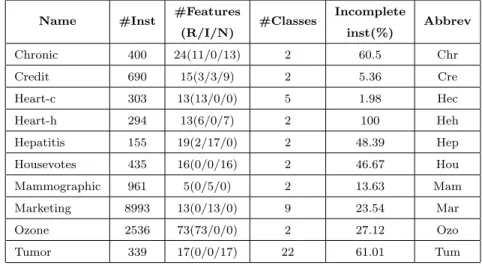
tory [3]. Table 3 summarises the main characteristics of the datasets includ- ing name, the number of instances, the number of features and their types (Real/Integer/Nominal), the number of classes and the percentage of incom- plete instances.
Table 3: Datasets used in the experiments
Name #Inst #Features (R/I/N)
#Classes Incomplete inst(%)
Abbrev
Chronic 400 24(11/0/13) 2 60.5 Chr
Credit 690 15(3/3/9) 2 5.36 Cre
Heart-c 303 13(13/0/0) 5 1.98 Hec
Heart-h 294 13(6/0/7) 2 100 Heh
Hepatitis 155 19(2/17/0) 2 48.39 Hep
Housevotes 435 16(0/0/16) 2 46.67 Hou
Mammographic 961 5(0/5/0) 2 13.63 Mam
Marketing 8993 13(0/13/0) 9 23.54 Mar
Ozone 2536 73(73/0/0) 2 27.12 Ozo
Tumor 339 17(0/0/17) 22 61.01 Tum
These benchmark datasets were carefully chosen to cover a wide-ranging col-
460
lection of problem domains. These tasks have various percentages of incomplete instances (incomplete instances range from 1.98% in the Hec dataset to 100%
in theHed dataset). These problems range from a small number of instances (Hep only has 155 instances) to a large number of instances (Mar has 8993
instances). These datasets also range between low to high dimensionality (Mam
465
only has 5 features whileOzo has 73 features). These problems encompass bi- nary and multiple-class classification tasks. We expect that these datasets can reflect incomplete problems of varying difficulty, size, dimensionality and type of features.
Ten-fold cross-validation [36] was used to separate each dataset into different
470
training and test sets. The ten-fold cross-validation process is stochastic, so it should be performed multiple times to eliminate statistical variations. Hence, the ten-fold cross-validation was independently performed 30 times on each dataset. As a result, there are 300 pairs of training set and test set for each dataset.
475
4.3. Parameter Settings 4.3.1. Imputation
The experiments used two imputation methods: kNN-based imputation and MICE, representing two types of imputation, single imputation and multiple imputation, respectively. With kNN-based imputation, for each incomplete
480
dataset, different values for the number of neighbors k (1, 5, 10, 15, 20) were checked to find the best value. The implementation of MICE using R language in [24] was used to run MICE where random forest was used as a regression method. The number of cycles was set as five and the number of imputed datasets was set 20 following the recommendation in [10].
485
4.3.2. Feature Selection
The proposed approach is a framework, so any feature selection method can be used to select relevant features. The experiments used a filter-based feature selection method because a filter method is often quicker and more general than a wrapper method. The Correlation Feature Selection (CFS) measure [31]
490
was used to evaluate feature subsets. The main reason is that CFS not only can evaluate the correlation between each feature with the class, but also can evaluate the uncorrelation between features in the feature subset. Moreover,
in many cases, CFS is as accurate as wrapper methods and it executes much faster than the wrapper methods [31]. An GA was used to search for feature
495
subsets because GA has been successfully applied to feature selection. Moreover, GA’s individuals can be represented by bitstrings which are suitable for feature selection, where 1 reflects selected features and 0 reflects unselected features.
The parameters of GA for feature selection were set as follows. The population size was set to 50 and the maximum number of generations was set to 100. The
500
crossover probability was set 0.9 and the mutation probability was set 0.1. CFS and GA were implemented under the WEKA [37].
4.3.3. Classifier learning Algorithms
In machine learning, classifier learning algorithms are often categorised into decision trees such as C4.5 [21], rule-based classifiers such as PART [38] ,
505
instance-based classifiers such ask nearest neighbour (kNN) [39], and function- based classifiers such as a multilayer perceptron (MLP) [1]. In recent years, ge- netic programming (GP) has been successfully applied to classification [40, 41].
Therefore, five classification algorithms (C4.5, PART, kNN, MLP and GP) were used to compare the proposed method with the other benchmark methods. The
510
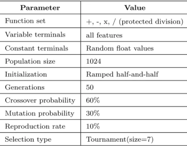
first four classification algorithms were implemented under the WEKA [37]. The implementation of GP in the experiment used the ECJ [42]. GP using a set of static thresholds as shown in [43] was used to decide class. Table 4 shows the parameters of GP for classification.
The proposed method,Ensemble[14] andEnsemble[16] automatically iden-
515
tify the number of classifiers from the training data. The number of classi- fiers in Ensemble[15] was set equally to the number of classifiers explored by Ensemble[14].
5. Results and Analysis
This section presents and discusses the experimental results. It first shows
520
the comparison on accuracy between the proposed method and the benchmark methods. It then presents the comparison between them on computation time.
Table 4: GP parameter settings
Parameter Value
Function set +, -, x, / (protected division) Variable terminals all features
Constant terminals Random float values Population size 1024
Initialization Ramped half-and-half
Generations 50
Crossover probability 60%
Mutation probability 30%
Reproduction rate 10%
Selection type Tournament(size=7)
Further analysis is also discussed to demonstrate the advantages of the proposed method.
5.1. Accuracy
525
5.1.1. Comparison Method
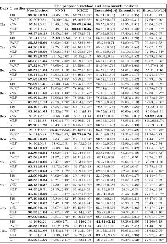
Table 5 shows the mean and standard deviation of classification accura- cies of the proposed method and the benchmark methods. The first column shows datasets, and the second column shows classification algorithms used in the experiments. “NewMethod” refers to the proposed method. The rest five
530
columns are the five benchmark methods. “kNNI” and “MICE”, respectively, are the benchmark methods using kNN-based imputation and MICE to esti- mate missing values as shown in Fig.1. “Ensemble[14]”, “Ensemble[16]” and
“Ensemble[15]” refer to the three ensemble benchmark methods in [14], [16]
and [15], respectively. The values in the table are the average classification ac-
535
curacy±standard deviation resulting from combining a classifier (row) with an approach to classification with incomplete data (column).
It is very important to choose a suitable statistical test to correctly evaluate the significance of the results. A multiple test rather than a pair test should be used to compare the proposed method with the multiple (five) benchmark
540
methods. Moreover, a non-parametric test rather a parametric test should be used because non-parametric tests do not require the normal distribution of
data as parametric tests. Therefore, the Friedman test [44], which is one of the most popular multiple non-parametric tests, is used to test the significance of the results. The test indicates that there exits significant differences between
545
the methods in each dataset and each classifier. Therefore, the Holm procedure [44], which is a post-hoc procedure, is used to perform pair tests between two methods. In Table 5, the symbol ↑ indicates that the proposed method is significantly better than the benchmark method. In contrast, the symbol ↓ shows that the proposed method is significantly worse than the benchmark
550
method.
5.1.2. Compare with Imputation Methods
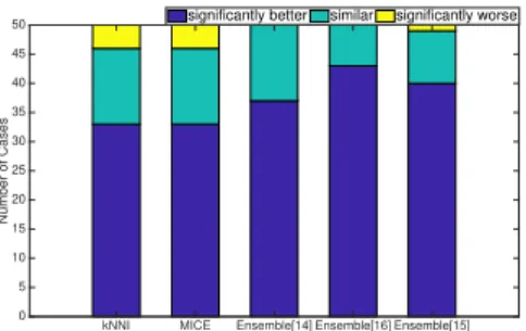
Fig. 3 shows the fraction of cases that the proposed method is significantly better or worse than the benchmark methods. It is clear from Fig 3 that the pro- posed method can achieve significantly better accuracy than using imputation
555
(kNNI andMICE) in most cases. The proposed method is significantly better than both kNNI and MICE in about 65% cases, and it is only significantly worse than both of them in 2 out of the 50 cases.
kNNI MICE Ensemble[14] Ensemble[16] Ensemble[15]
0 5 10 15 20 25 30 35 40 45 50
Number of Cases
significantly better similar significantly worse
Figure 3: The comparison between the proposed method and each of the benchmark methods on all the classification algorithms.
The proposed method is more accurate than the imputation methods be- cause it incorporates feature selection to remove redundant and irrelevant fea-
560
tures, which helps to improve classification accuracy. Furthermore, the proposed method can construct multiple classifiers, which can be more comprehensive and generalise better than constructing a single classifier. Therefore, the proposed method can classify new instances better than the imputation methods.
Table 5: Mean and standard deviation of classification accuracies.
Data Classifier The proposed method and benchmark methods
NewMethod kNNI MICE Ensemble[14] Ensemble[16] Ensemble[15]
Chr
J48 99.10±0.33 99.05±0.35 97.53±0.62↑ 94.21±0.46↑ 94.18±0.35↑ 97.41±0.73↑
PART 99.30±0.34 99.20±0.53 98.40±0.68↑ 94.28±0.49↑ 94.20±0.31↑ 97.60±0.60↑
kNN 97.78±0.28 98.40±0.28↓ 98.65±0.30↓ 93.55±0.36↑ 93.95±0.31↑ 98.06±0.69↓
MLP 96.92±0.47 98.48±0.44↓ 99.00±0.35↓ 93.93±0.33↑ 93.90±0.40↑ 96.50±0.67↑
GP 98.97±0.29 97.95±0.48↑ 97.95±0.52↑ 97.62±0.31↑ 97.46±0.34↑ 96.20±0.65↑
Cre
J48 85.34±0.54 85.38±0.52 85.31±0.58 85.06±0.67↑ 84.98±0.76↑ 80.24±1.26↑
PART 85.33±0.66 83.92±0.92↑ 83.82±0.86↑ 85.26±0.71 84.80±0.77↑ 79.38±1.58↑
kNN 84.20±0.81 82.75±0.53↑ 82.76±0.62↑ 83.46±0.61↑ 82.46±0.54↑ 74.62±1.59↑
MLP 86.17±0.59 83.02±0.94↑ 83.25±0.78↑ 85.18±0.62↑ 85.10±0.56↑ 77.19±2.84↑
GP 86.19±0.52 86.15±0.62 85.95±0.62 86.03±0.49 85.55±0.52↑ 79.78±1.46↑
Hec
J48 58.06±1.55 54.26±2.08↑ 54.09±1.98↑ 55.17±1.74↑ 53.10±1.49↑ 56.67±0.96↑
PART 57.32±1.77 53.65±2.13↑ 53.75±1.45↑ 54.00±1.71↑ 51.55±2.08↑ 56.57±1.06 kNN 55.51±1.83 54.82±1.13↑ 54.57±1.18↑ 54.74±1.05↑ 54.61±1.35↑ 55.11±1.40 MLP 58.34±1.45 53.63±1.53↑ 54.19±1.96↑ 54.21±1.50↑ 52.98±1.57↑ 57.24±1.07↑
GP 57.83±0.92 56.73±1.05↑ 56.29±1.05↑ 56.77±1.17↑ 57.21±1.42↑ 56.73±0.58↑
Heh
J48 78.92±1.51 78.33±1.56 78.25±1.39↑ 76.86±1.41↑ 76.76±1.49↑ 63.50±6.32↑
PART 79.02±1.47 76.92±2.07↑ 78.80±1.19↑ 77.11±1.44↑ 77.61±1.50↑ 63.79±7.02↑
kNN 80.11±1.50 76.63±1.33↑ 76.21±1.75↑ 74.69±1.30↑ 74.82±1.24↑ 62.38±5.72↑
MLP 80.50±1.30 77.96±1.56↑ 78.58±1.63↑ 76.93±1.43↑ 77.23±1.48↑ 63.78±5.95↑
GP 81.55±1.13 79.76±1.70↑ 80.34±1.42↑ 79.36±0.90↑ 79.63±1.10↑ 72.83±2.56↑
Hep
J48 82.19±1.46 78.55±2.05↑ 80.01±2.25↑ 79.80±1.76↑ 80.98±1.58↑ 81.52±1.52 PART 82.16±1.64 79.32±2.75↑ 82.11±1.85 80.75±1.83↑ 80.69±1.92↑ 82.04±1.91 kNN 80.49±2.68 80.66±1.40 80.21±1.44 80.17±0.92 77.94±1.01↑ 80.82±2.31 MLP 83.01±1.88 81.61±1.77↑ 82.56±1.24↑ 80.16±1.23↑ 78.85±2.18↑ 83.16±1.74 GP 82.70±1.70 80.43±2.81↑ 80.45±1.90↑ 80.54±1.40↑ 78.45±1.33↑ 82.59±2.00
Hou
J48 95.00±0.35 96.31±0.52↓ 96.15±0.54↓ 93.69±0.37↑ 93.70±0.39↑ 90.97±0.72↑
PART 94.94±0.38 95.59±0.63↓ 95.72±0.79↓ 94.14±0.35↑ 94.31±0.44↑ 91.26±0.82↑
kNN 95.40±0.39 92.33±0.55↑ 93.01±0.34↑ 90.83±0.41↑ 91.43±0.42↑ 91.43±0.77↑
MLP 94.70±0.47 94.82±0.51 94.72±0.65 93.45±0.53↑ 93.98±0.48↑ 91.19±0.74↑
GP 95.14±0.59 95.08±0.66 95.11±0.48 94.32±0.33↑ 94.24±0.32↑ 91.64±0.85↑
Mam
J48 82.86±0.52 81.92±0.54↑ 82.24±0.65↑ 82.57±0.46↑ 82.33±0.49↑ 79.68±1.53↑
PART 82.58±0.52 81.57±0.52↑ 81.71±0.49↑ 82.18±0.64 82.13±0.55 79.74±0.79↑
kNN 80.31±0.60 75.47±0.69↑ 75.93±0.66↑ 78.37±0.66↑ 79.64±0.71↑ 79.89±1.16 MLP 83.11±0.43 82.72±0.63 82.97±0.49 82.99±0.36 82.95±0.45 79.73±1.05↑
GP 82.52±0.53 79.72±1.12↑ 79.99±0.68↑ 82.25±0.53↑ 82.46±0.69 77.04±2.15↑
Mar
J48 33.90±0.30 30.02±0.56↑ 30.01±0.41↑ 33.32±0.40↑ 33.43±0.37↑ 31.14±0.51↑
PART 33.53±0.34 28.71±0.33↑ 28.83±0.42↑ 32.82±0.37↑ 32.82±0.42↑ 30.84±0.63↑
kNN 33.13±0.37 27.30±0.42↑ 27.55±0.39↑ 29.34±0.38↑ 29.71±0.38↑ 30.77±0.76↑
MLP 34.35±0.21 32.15±0.45↑ 32.40±0.38↑ 34.26±0.22 34.24±0.29 30.18±0.84↑
GP 31.45±0.20 30.51±0.47↑ 30.47±0.50↑ 31.34±0.24 31.32±0.38 27.87±1.07↑
Ozo
J48 97.10±0.04 95.84±0.82↑ 95.90±0.40↑ 96.44±0.24↑ 96.83±0.21↑ 83.47±0.95↑
PART 97.10±0.02 95.47±1.23↑ 95.86±0.44↑ 96.89±0.16↑ 96.93±0.17↑ 83.43±0.99↑
kNN 96.50±0.19 95.07±0.62↑ 95.15±0.32↑ 95.35±0.31↑ 96.28±0.26↑ 83.17±0.74↑
MLP 96.35±1.04 96.07±0.59↑ 96.34±0.27 96.28±0.19 96.30±0.17 83.70±1.10↑
GP 97.09±0.05 95.81±0.72↑ 95.90±0.40↑ 96.44±0.24↑ 96.83±0.21↑ 83.61±0.97↑
Tum
J48 41.16±2.24 41.08±2.71 41.24±2.05 42.32±2.12 38.38±2.59↑ 31.26±3.18↑
PART 40.55±2.06 40.17±1.78 40.49±1.76 40.35±1.99 37.46±2.41↑ 31.40±3.50↑
kNN 39.12±1.96 38.43±1.74↑ 38.41±1.98↑ 38.13±1.66↑ 36.05±1.86↑ 31.62±2.95↑
MLP 38.85±2.01 39.38±1.62 39.79±2.29 39.83±2.09 36.40±1.96↑ 32.97±2.20↑
GP 31.59±1.56 30.86±2.41↑ 30.83±1.90 31.55±1.88 30.39±1.52↑ 27.61±1.49↑
5.1.3. Compare with Other Ensemble Methods
565
As also can be seen from Fig. 3 that the proposed method also can achieve significantly better accuracy than the benchmark ensemble methods in most cases. The proposed method is significantly more accurate than the benchmark ensemble methods in at least 75% cases, and it is only significantly less accurate than theensemble[15] in 1 out of the 50 cases.
570
The proposed method is more accurate than the other benchmark ensem- ble methods because it uses a powerful imputation to provide complete data for the training process rather than working on incomplete training data as Ensemble[14] and Ensemble[16]. The second reason is that feature selection helps to further improve the training data of the proposed method. Moreover,
575
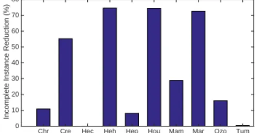
by removing redundant and irrelevant features, feature selection helps to re- duce the number of incomplete instances in the application process as shown in Fig.4. As a result, the proposed method can more frequently choose applicable classifiers to classify incomplete instances than the other ensemble methods.
Chr Cre Hec Heh Hep Hou Mam Mar Ozo Tum 0
10 20 30 40 50 60 70 80
Incomplete Instance Reduction (%)
Figure 4: The percentage of incomplete instance reduction by using feature slection.
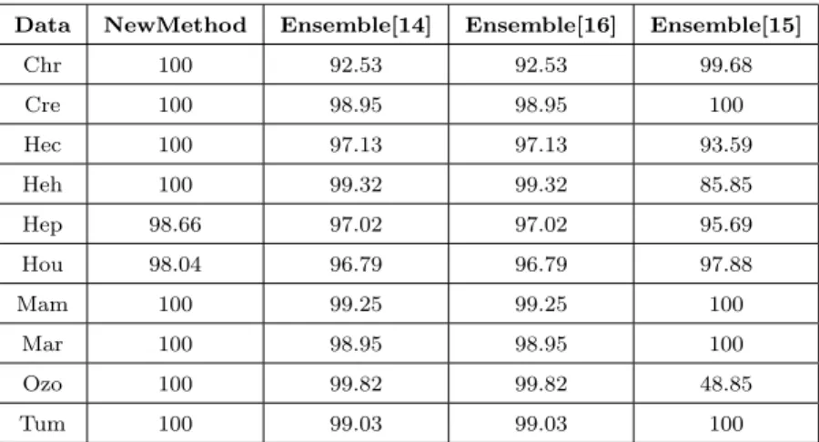
Table 6 shows the percentage of incomplete instances which can be clas-
580
sified by the ensemble methods. It is clear from Table 6 that the proposed method can classify all incomplete instances on 8 out of 10 datasets and clas- sify almost all incomplete instances on the other 2 datasets. In contrast, the other ensemble methods cannot well classify incomplete instances. Especially, Ensemble[15] only can classify 85.85% and 48.85% incomplete instances on the
585
Heh andOzo datasets, respectively, becauseEnsemble[15] randomly generates missing patterns instead of finding missing patterns in the training data as the other ensemble methods.
Table 6: The percentage of incomplete instances are classified by ensemble methods.
Data NewMethod Ensemble[14] Ensemble[16] Ensemble[15]
Chr 100 92.53 92.53 99.68
Cre 100 98.95 98.95 100
Hec 100 97.13 97.13 93.59
Heh 100 99.32 99.32 85.85
Hep 98.66 97.02 97.02 95.69
Hou 98.04 96.79 96.79 97.88
Mam 100 99.25 99.25 100
Mar 100 98.95 98.95 100
Ozo 100 99.82 99.82 48.85
Tum 100 99.03 99.03 100
5.1.4. Further Comparison
As can be seen from Table 5 that the proposed method can obtain better
590
accuracy than the benchmark methods not only on datasets with a small number of incomplete instances, but also on datasets with a large number of incomplete instances. For instance, the proposed method achieves the best accuracy onHec dataset containing only 5.36% incomplete instances and also on Heh dataset with 99.65% incomplete instances.
595
Fig. 5 shows the fraction of cases that the proposed method is significantly better or worse than the other methods on each classifier. Fig. 5 shows that with any of the classifiers, the proposed method can significantly outperform the other methods in most cases. Moreover,J48 andGP can get more benefits from the proposed method. The reason is likely that a filter feature selection
600
often removes irrelevant and redundant features, but it may keep redundant features. J48 andGPcan perform feature selection while constructing classifiers [45, 46]. Therefore, by further removing redundant and irrelevant features, these classifiers can be more tolerant of missing values [12].
In summary, the proposed method can obtain significantly better accuracy
605
than the benchmark methods in almost all cases when combining with any of the classification algorithms.