Appendix B lists additional language features of the Julia language that are not used by the code examples in this book. The remainder of this chapter is structured as follows: In Section 1.1 we present a brief overview of the Julia language.
Language Overview
LANGUAGE OVERVIEW 5 the commercial company Julia Computing provides services and support for schools, universities,
Line 7, is the body of the loop where println() is used to print various arguments. The expression from the last line of each code block, unless terminated by a ";", is presented as output.
LANGUAGE OVERVIEW 7
Although Julia is fast and efficient, we do not specifically focus on execution speed and performance in most of this book. When the using command of a given package is called for the first time (during a session), you can sometimes wait a few seconds for the package to compile.
LANGUAGE OVERVIEW 9 into more complicated projects, many repetitions of the same code block may merit profiling and
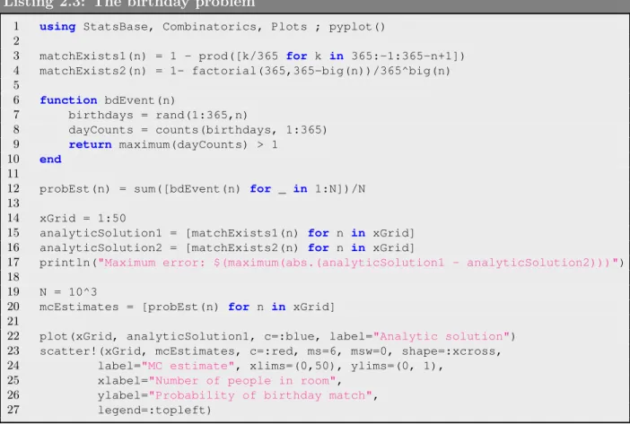
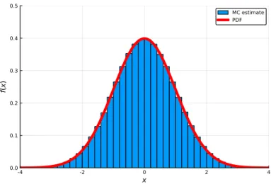
INTRODUCING JULIA - DRAFT As can be seen, the output gives the same estimate for the interval containing 98% of the means. This is not part of the Julia language, but rather decorates the name of the function.
SETUP AND INTERFACE 11
Setup and Interface
A common way to run Jupyter for Julia is to use the Anaconda Python distribution, which installs a Jupyter notebook server locally. Note that JuliaBox is a paid service, while running a Jupyter notebook on your own local machine is free.
SETUP AND INTERFACE 13
CSV.jl is a utility library for working with CSV and other delimited files in Julia. Dates.jl is one of Julia's standard libraries and provides support for working with dates and times.
SETUP AND INTERFACE 15 HCubature.jl is an implementation of multidimensional “h-adaptive” (numerical) integration
StatsBase.jl provides basic statistics support by implementing a variety of statistics-related functions, such as scalar statistics, higher-order moment computation, counts, ranks, covariance, sampling, and cumulative distribution function estimation.
Crash Course by Example
CRASH COURSE BY EXAMPLE 17 with matrices and randomness (Markov chain), and show how it can be interfaced with the web and.
CRASH COURSE BY EXAMPLE 17 with matrices and randomness (Markov chain), and show how one can interface with the web and
This exclamation mark adorns the name of the function and tells us that the function argument, a, will be modified (sorted in place with no memory copy). We then use this function as an argument to the find_zeros() function, which then returns the roots of the original polynomial.
CRASH COURSE BY EXAMPLE 19 Listing 1.6 shows our approach. Note that for our example it is straightforward to solve the
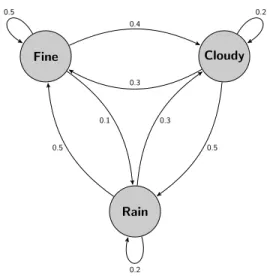
That is, at steady state, what percentage of the time is the weather in state 1,2, or 3. This linear system of equations can be rearranged into a system of 3 equations and 3 unknowns by realizing that one of the equations within πP = π is redundant.
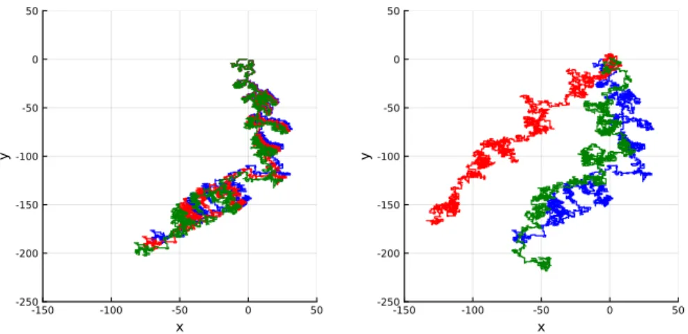
CRASH COURSE BY EXAMPLE 21 4. We run a simple Monte Carlo simulation (see also Section 1.5) by generating random values
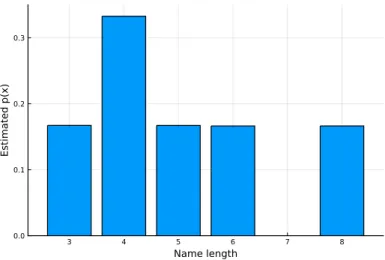
Also notice that during the normalization in line 19, we use the L1 norm which is basically the sum of the absolute values of the vector. In particular, we want to look at the occurrences of some common words in all of his popular texts and present a count of some of the more common words.
CRASH COURSE BY EXAMPLE 23 Now with some basic understanding of JSON, we can proceed with our example. The code in
Plots, Images and Graphics
PLOTS, IMAGES AND GRAPHICS 25 bar() - Used for plotting bar graphs
In line 3, we define a function of two variables with real values f(), which is the main object of this example. Finally, in line 21, the three previous subplots are plotted together as one image via the plot() function.
PLOTS, IMAGES AND GRAPHICS 27
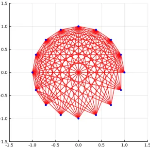
In this case, we construct a set of equally spaced nodes around the unit circle, given the integer number of nodes, n. To add another dimension to this example, we obtain points around the unit circle by considering complex numbers. We then use the real and imaginary parts of zn to get the horizontal and vertical coordinates for each vertex, which evenly distributes n points on the unit circle.
PLOTS, IMAGES AND GRAPHICS 29
RANDOM NUMBERS AND MONTE CARLO SIMULATION 31
Random Numbers and Monte Carlo Simulation
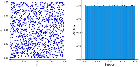
Then, if we want to have a pseudorandom number in the range [0,1] (represented by a floating point number), we normalize via,. As can be seen from the output, setting the seed to 1974 produces the same sequence.
RANDOM NUMBERS AND MONTE CARLO SIMULATION 33
Most of the code examples in this book use Us number of iterations in a Monte Carlo simulation. Number theory and related fields play a central role in the mathematical study of the generation of pseudorandom numbers, the interior of which is determined by the singularities f(·) of (1.5).
RANDOM NUMBERS AND MONTE CARLO SIMULATION 35
Our interest in mentioning the Mersenne Twister is because in Julia we can create an object that represents a random number generator implemented via this algorithm. By creating random number generator objects, you can have more than one random sequence in your application that essentially work simultaneously.
RANDOM NUMBERS AND MONTE CARLO SIMULATION 37 Listing 1.16: Random walks and seeds
Integration with Other Languages
INTEGRATION WITH OTHER LANGUAGES 39
TextBlob's sentiment analyzer outputs a tuple of values, where the first value is the polarity of the sentence (an assessment from positive to negative) and the second value is an assessment of subjectivity (actual to subjective). In line 12, a term is used to print the sentiment field for each phrase in blob.
INTEGRATION WITH OTHER LANGUAGES 41 Other Integrations
This chapter is structured as follows: In Section 2.1, we examine the basic setup of randomized experiments with a few examples. In section 2.2 we examine the work with sets in Julia as well as probability examples dealing with associations of events.
Random Experiments
Finally, we count the number of true values by summing all the comprehension elements via sum(). In this case, 4 characters are matched (shown in bold), so the event is logged.
RANDOM EXPERIMENTS 47
RANDOM EXPERIMENTS 49
RANDOM EXPERIMENTS 51
This is illustrated in Figure 2-3, where it is clear that there are many possible paths the ant could take. That is, what is the probability that the ant will stay on or above the diagonal if it travels from (0,0) to (n, n).
RANDOM EXPERIMENTS 53 case where there is no option for the ant (i.e. it hits the east or north border) then it simply
WORKING WITH SETS 55
Working With Sets
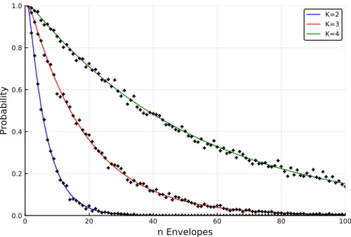
The probability of each of the business cards ending up in the right envelope is easy to figure out. However, what is the probability that each of the business cards ends up in the wrong envelope?
WORKING WITH SETS 61
Note that in this for loop there is no need to keep a count of the loop iteration count, so for clarity we use underscores in line 7. Note the use of element-wise comparison.>, which results in an array of boolean values that can be summed.
Independence
Conditional Probability
To help illustrate this further, consider a player who rolls the die without showing us the result, and then tells us the following: "The sum is greater than or equal to 10. Let Abe be the event of a manufacturing error, and assume that it depends on the number of dust particles via,.
Bayes’ Rule
As an example, take a communication channel involving a stream of transmitted bits (0s and 1s) where 70% of the bits are 1 and the rest 0. The channel is imperfect due to physical disturbances such as interfering radio signals, and in addition, the received bits are sometimes distorted.
BAYES’ RULE 67
If the player accepts Policy I, she always sticks to her initial guess, regardless of the GSH action. However, if she accepts Policy II, she always switches after the GSH reveals an empty door.
BAYES’ RULE 69 Listing 2.13: The Monty Hall problem
The chapter is organized as follows: In Section 3.1 we introduce the concept of a random variable and its probability distribution. In Section 3.4 we focus on the Julia Distributions package, which is useful when working with probability distributions.
Random Variables
Mathematically, a random variable X is a function of the sample space, Ω, and assumes integer, real, complex, or even a vector of values. This is followed by Section 3.6, where we explore some continuous distributions along with additional concepts such as hazard rates and more.
RANDOM VARIABLES 73
There are additional descriptors of probability distributions other than PMF and PDF, and these are discussed further in Section 3.3. In line 3 we define an array that specifies the PMF of our discrete distribution, and in lines 6 and 9 we define functions that specify the PDFs of our continuous distributions.
Moment Based Descriptors
MOMENT BASED DESCRIPTORS 75
Note that the above expression does not require explicit knowledge of the distribution of Y, but rather uses the distribution (PMF or PDF) of X. The variance of the random variable X, often denoted as Var(X) or σ2, is a measure of the spread or dispersion of the distribution of X.
MOMENT BASED DESCRIPTORS 77
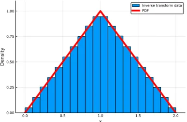
It can be seen from the output that the mean of the distribution Y is the same as the variance of X. It can be observed that the histogram on the left approximates the PDF of our triangular distribution, while the histogram on the right approximates the distribution of the new variable Y.
MOMENT BASED DESCRIPTORS 79 and the strong law of large numbers. In both cases, a sequence of independent and identically
Functions Describing Distributions
FUNCTIONS DESCRIBING DISTRIBUTIONS 81
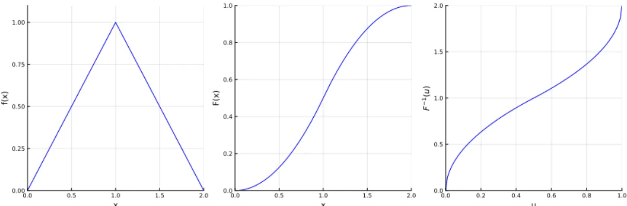
In cases where the CDF is continuous and strictly increasing over all values, the inverse, F−1(·) is well defined and can be found via the equation,. In more general cases where the CDF is not necessarily strictly increasing and continuous, we can still define the inverse CDF via , .
FUNCTIONS DESCRIBING DISTRIBUTIONS 83
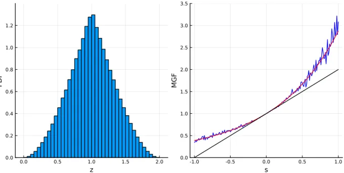
In this case it is known that the MGF of Z is the product of the MGFs of X1 and X2. To then calculate the moment, one can simply evaluate the derivative of the MGF at s=0.
FUNCTIONS DESCRIBING DISTRIBUTIONS 85
In line 8, we generate observations for Z by performing element-wise summation of the values in our arrays data1anddata2. The rest of the code uses the data and the defined functions to generate Figure 3.6.
Distributions and Related Packages
Note that the third argument of the TriangleDistribution() function is the location of the "peak" of the triangle (or the mode of the distribution). In lines 12-13 we define the function mgfPuntEst(), which roughly estimates the MGF at point s.
DISTRIBUTIONS AND RELATED PACKAGES 87
You can search for mean(), median(), var() (variance), std, (standard deviation), skewness() and kurtosis(). You can also search for the minimum and maximum value in the distribution support viaminimum() and maximum() respectively.
DISTRIBUTIONS AND RELATED PACKAGES 89 In Listing 3.11 we look at another example, where we generate random observations from a dis-
To see why the method works, consider a uniform random variable U and apply the inverse probability transformation F−1(·) to it. However, in Listing 3.12 below, we illustrate how to use the inverse probability transformation with the results in Figure 3-8.
FAMILIES OF DISCRETE DISTRIBUTIONS 91
Families of Discrete Distributions
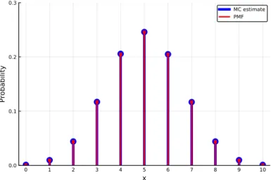
The parameters and support for each distribution are presented in more detail later in this section. Listing 3.14 simulates N rolls of a die and then calculates and plots the proportion of times each possible outcome occurs along with the PMF.
FAMILIES OF DISCRETE DISTRIBUTIONS 93
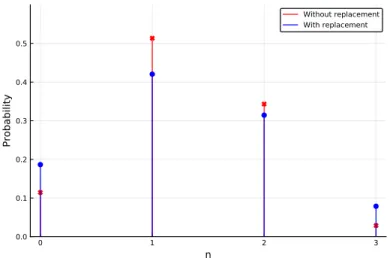
In line 11, we use counts() from the StatsBase package to count the number of times each outcome for 0:nheads occurred. Note that the binomial distribution describes the part of the fishing example in Section 2.1 where we sample with replacement.
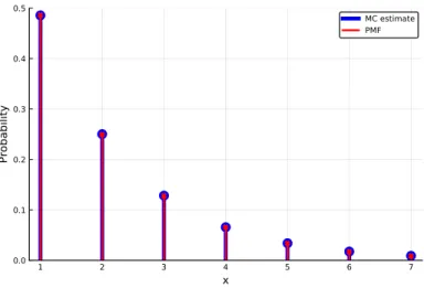
FAMILIES OF DISCRETE DISTRIBUTIONS 95 Geometric Distribution
Similar to the geometric case, there is an alternative version of the negative binomial distribution. That is, we determine the probabilities that will occur until the fifth success (or win).
FAMILIES OF DISCRETE DISTRIBUTIONS 97
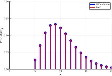
Here the parameter L is the population size, and K is the number of successes present in the population (this implies that L - K is the number of failures present in the population). We consider several of these cases, where the only difference between each is the number of successes, K, (goldfish) in the population.
FAMILIES OF DISCRETE DISTRIBUTIONS 99
A Poisson process is a stochastic process (random process) that can be used to model the occurrence of events over time (or more generally in space). A full description and analysis of the Poisson process is beyond our scope, but we provide an overview of the basics.
FAMILIES OF DISCRETE DISTRIBUTIONS 101
Families of Continuous Distributions
FAMILIES OF CONTINUOUS DISTRIBUTIONS 103
This alludes to the fact that exponential random variables are continuous analogs of geometric random variables. In Listing 3.22 we present a comparison between the PMF of the bottom of an exponential random variable and the PMF of the geometric distribution discussed in Section 3.5.
FAMILIES OF CONTINUOUS DISTRIBUTIONS 105
To introduce this distribution, consider the following example, where the lifetime of light bulbs is exponentially distributed with meanλ−1. It can be seen that for a gamma random variable, the SCV is 1/α and for our light bulb example above, SCV(T) = 1/n.
FAMILIES OF CONTINUOUS DISTRIBUTIONS 107
In line 7, the Gamma() function is used in conjunction with Comprehension to generate the Gamma distribution for each of our examples. By focusing on the normalizing constant, we gain further insight into the mathematical function gamma Γ(·), which is a component of the previously discussed gamma distribution.
FAMILIES OF CONTINUOUS DISTRIBUTIONS 109 This is the recursive definition of factorial. The gamma function exhibits similar properties, and
The Weibull distribution is naturally defined by the hazard rate by considering hazard rate functions that have a specific simple form. If α= 1, the hazard rate is constant, in which case the Weibull distribution is effectively an exponential distribution with degree λ.
FAMILIES OF CONTINUOUS DISTRIBUTIONS 111
It is commonly exhibited due to the central limit theorem, which is covered in more depth in Section 5.3. These are exactly the inflection points of the normal PDF (points where the function switches from being locally convex to locally concave or vice versa).
FAMILIES OF CONTINUOUS DISTRIBUTIONS 113
Hence the implication is that since we know how to generate exponential random variables via −λ1log(U) whereU ∼uniform(0,1), then we can generate Rayleigh random variables by applying a square root. As we see in the next example, this property provides a method to generate normal random variables.
FAMILIES OF CONTINUOUS DISTRIBUTIONS 115
In line 4, we define a functionZ() which implements the Box-Muller transform and generates a single standard normal random variable. For each shot from the laser, a point, X, can be measured horizontally on the ground from the point over which the drone hovers.
FAMILIES OF CONTINUOUS DISTRIBUTIONS 117
Line 2 sets the seed of the random number generator so that the same stream of random numbers is generated each time. In line 5, we create data, an array of n Cauchy random variables constructed by the angle mechanism described and illustrated in Figure 3.22.
Joint Distributions and Covariance
JOINT DISTRIBUTIONS AND COVARIANCE 119
This grid is then used to obtain a rough approximation of the integral in line 8, with the result printed in line 9. Similarly, the nested integral (3,25) is approximated via two Riemann sums in line 11, with the result printed in line 12.
JOINT DISTRIBUTIONS AND COVARIANCE 121 Covariance and Vectorized Moments
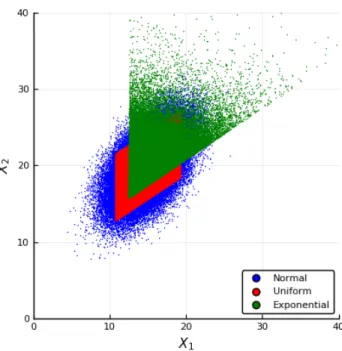
Now say you want to create an n-dimensional random vector Y with some specified mean vector µY and covariance matrixΣY. Listing 3.32 generates random vectors with this mean vector and covariance matrix using three alternative forms of zero-mean, identity-covariance matrix random variables.
JOINT DISTRIBUTIONS AND COVARIANCE 125
Single sample over time (time series): The configuration of the data has the form: xt1, xt2,. The first is called call by value and describes a situation where the code implementing f() gets a copy of the variable x.
WORKING WITH DATA FRAMES 131
Working with Data Frames
In line 4, thesize() function is used to return the number of rows and columns of the data frame as a tuple. In line 7, describe() is used to create a data frame with a summary of the data in each column of the input data frame (data in our case).
WORKING WITH DATA FRAMES 133 Referencing Data
However, by default the columns of a data frame are immutable, meaning that the values in them cannot be changed. One way to do this is by including copycols=true when creating a dataframe from a csv file.
WORKING WITH DATA FRAMES 135
This is the example in lines 15-19 where we create a data frame with a column named X consisting of strings. Now let's take a closer look at the case where there are missing values in the data frame.
WORKING WITH DATA FRAMES 137
WORKING WITH DATA FRAMES 139
The columns referred to in the calculations are placed to the left of '=>', only in our case: Price is used. Note that => is used to define aPair and -> is used to define an anonymous function.
WORKING WITH DATA FRAMES 141 A Cleaning and Imputation Example
In lines 10-11, dropmissing() and by() are used to calculate the average price of each group, excluding rows with missing values. In lines 16-18 if the price entry is missing, the grade is used to return the corresponding value stored in the dictionary.
Summarizing Data
In lines 4-5, we check if there are any rows with missing values in both the :Grade and :Price columns, and we remove them if present. Similarly, in lines 19-21 if the grade entry is missing, thennearIndx() function is used to find the index of the nearest value in grPr based on the price in data, and then missing is replaced by the corresponding grade.
SUMMARIZING DATA 143 is given by,
The range and IQR are measures of dispersion, meaning that the larger their size, the greater the dispersion of the data. If all observations are constant, s2 = 0, otherwise s2 >0, and the larger it is, the more spread we have in the data.
SUMMARIZING DATA 145
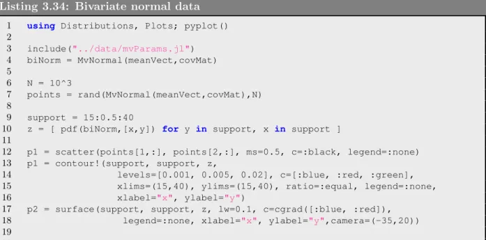
In Listing 4.12, we enter a weather observation data set containing pairs of temperature observations (see Section 3.7). Note that this file is used as input to Listing 3.34 at the end of Chapter 3.
SUMMARIZING DATA 147
We now illustrate several alternative ways of computing the sample covariance and sample correlation in Listing 4.13 below. In addition to the cov(), cor(), mean(), and std() functions, the listing also illustrates the use of thezscore() function from StatsBase.
PLOTS FOR SINGLE SAMPLES AND TIME SERIES 149
Plots for Single Samples and Time Series
First indicate the support of the observations via [`, m]where` is the minimum observation and miss is the maximum observation. Thus, an alternative representation is via a histogram function h(x) which is a scaled graph of the frequencies f1 .
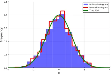
PLOTS FOR SINGLE SAMPLES AND TIME SERIES 151 discuss these methods here. Throughout this book we use the histogram() function from Plots
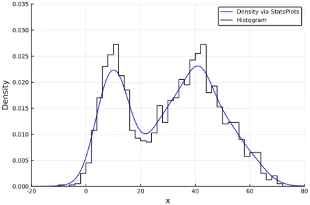
Initially, a random (unobserved) variable determines which subpopulation is used, and then a sample is drawn from that subpopulation. Moreover, the probability density function of the mixture is a convex combination of the probability density functions of each of the subpopulations.
PLOTS FOR SINGLE SAMPLES AND TIME SERIES 153
This again implies that KDE (4.8) consists of a superposition of highly concentrated functions, one for each observation. It generates Figure 4.3, where the left plot compares the KDE with the underlying PDF of the mixture, and the right plot shows the effect of changing the bandwidths.
PLOTS FOR SINGLE SAMPLES AND TIME SERIES 155 Listing 4.16: Kernel density estimation
In Listing 4.17 we use synthetic data from the same mixture distribution as in the two previous examples. The first few lines of the code block are similar to the previous mixed distribution examples.
PLOTS FOR SINGLE SAMPLES AND TIME SERIES 157
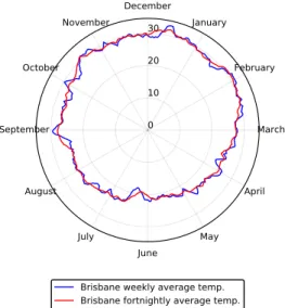
The top left plot presents two time series of temperature data in the adjacent locations of Brisbane and Gold Coast Australia. The bottom left plot is a time series of the differences in temperatures between Brisbane and Gold Coast.
PLOTS FOR SINGLE SAMPLES AND TIME SERIES 159
In lines 3-5 we read the data and create the brisbane and goldcoast arrays describing the temperatures at these respective locations. A variation of the radial chart is the radar chart, which is often used to visualize the levels of different categorical variables in a plot.
Plots for Comparing Two or More Samples
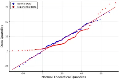
PLOTS FOR COMPARING TWO OR MORE SAMPLES 163 Listing 4.21: Q-Q Plots
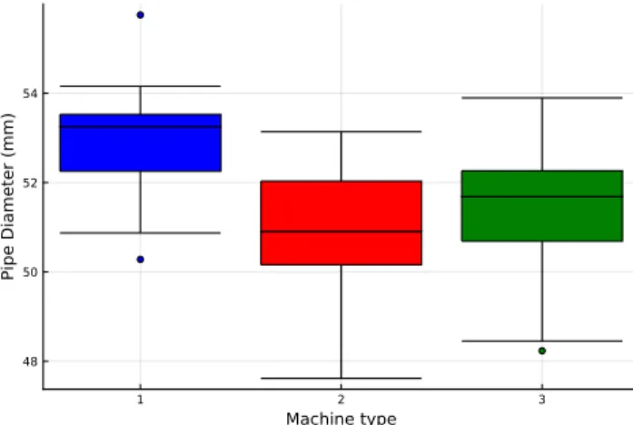
Lines 3-5 load the data files for each of the machines and store the data as separate arrays. It is similar to the box plot, but the shape of each sample is represented by a mirrored kernel density estimate of the data.
PLOTS FOR MULTIVARIATE AND HIGH DIMENSIONAL DATA 165
Plots for Multivariate and High Dimensional Data
It consists of taking each possible pair of variables and sketching a scatterplot for that pair. As with any scatterplot, data in scatterplot matrices can also be colored or labeled.
PLOTS FOR MULTIVARIATE AND HIGH DIMENSIONAL DATA 167
Cell colors indicate size, where typically, the 'warmer' the color, the higher the value. The right plot is for synthetic data based on a bivariate normal distribution fitted to that data, with the actual parameters fitted in Listing 4.12.
PLOTS FOR MULTIVARIATE AND HIGH DIMENSIONAL DATA 169
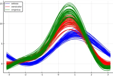
The first argument, :Species, specifies how to group the data, while the second argument specifies which variables to include in the calculation, in this case columns 1 through 4.
PLOTS FOR THE BOARD ROOM 171
Plots for the Board Room
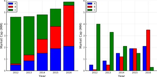
Listing 4.28 summarizes the data from companyData.csv, and presents the total market capitalization of each company for each year through a stacked bar plot and clustered bar plot. In line 5, reshape() is used to reshape the market cap data from a single column to a 5×3 array, with the rows representing years and columns representing companies.
WORKING WITH FILES AND REMOTE SERVERS 173
Working with Files and Remote Servers
In Listing 4.30, we created a function that searches a text document for a specific keyword, then saves each line of text containing that keyword to a new text file, along with the corresponding line number. Line 14 uses lineSearch to search the "earth.txt" file for the keyword "water", storing the line numbers and text in the "waterLines.txt" file.
WORKING WITH FILES AND REMOTE SERVERS 175 Searching for Files in a Directory
Point Estimate - Determination of a single value (or vector of values) that represents the best estimate of the parameter(s). In Section 5.3 we examine the central limit theorem, which justifies the ubiquity of the normal distribution.
A Random Sample
CONCEPTS OF STATISTICAL INFERENCE - DRAFT Most of the point estimates, confidence intervals, and hypothesis tests introduced and performed in this book are elementary. This chapter is structured as follows: In Section 5.1, we introduce the concept of a random sample along with the distribution of statistics such as the distribution of the sample mean and sample variance.
A RANDOM SAMPLE 179
This means that for an exponential distribution with degree λ, the mean is λ−1 and the variance is λ−2. In lines 22–26, we create histograms of the sample means and sample variances using 200 and 600 bins, respectively.
Sampling from a Normal Population
We can see that the estimated expected values of our simulated data are good approximations of the mean and variance parameters of the underlying exponential distribution.
SAMPLING FROM A NORMAL POPULATION 181
Observe the PDF of a scaled chi-square distribution using the pdf() and Chisq() functions in line 28. Finally, notice the PDF of the T statistic (T), which is described by a T distribution, is plotted using theTDist() function in line 33.
SAMPLING FROM A NORMAL POPULATION 183
SAMPLING FROM A NORMAL POPULATION 185
In Listing 5.4 below, we first illustrate the validity of the representation (5.4) by generating T-distributed random variables using a standard normal and a chi-square random variable. In line 6, we specify the function myT() which generates a t-distributed random variable using a standard normal and a chi-square random variable, as in (5.4).
SAMPLING FROM A NORMAL POPULATION 187
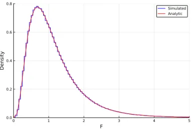
A single F statistic is then calculated from the ratio of the sample variances of these two groups. The rest of the code creates the figure where in line 18 the FDist() constructor is used to create an F-distribution with the parameters n1-1andn2-2.
THE CENTRAL LIMIT THEOREM 189
The Central Limit Theorem