After many years of success, she left friendly Europe for the next grand tour of her life, to the host of the most advanced materials science – the United States – interestingly enough, not to another industrial super-organization like Thomson, but to a university, where she could share her experiences and shape the next generations. Perhaps you will hear - as I did - the whisper of Professor Razeghi's modestly hidden powerful message: the only thing keeping you from performing miracles in the tournament with nature is yourself.
Introduction
Spectroscopic Emission lines and Atomic Structure
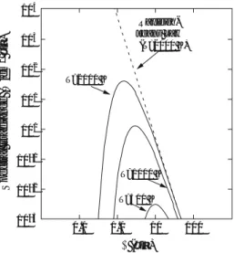
The coulombic force between the electron and the nucleus gives this acceleration, as illustrated in fig. 1.2. The second series occurs when the electron falls from higher levels to the levels with n¼2 (Balmer series) and n¼3 (Paschen series), as shown in Fig.1.1.
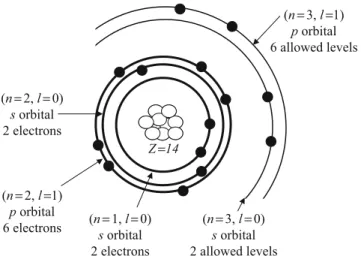
Atomic Orbitals
1.4 (a) The precise spherical orbit of an electron in the first Bohr orbit, for which the radius is a0¼0.52917 Å, as calculated by Bohr's model. b) The electron probability density pattern for the comparable atomic orbital using a quantum mechanical model. It is the value of this quantum number n that determines the size and energy of the principal orbitals.
Structures of Atoms with Many Electrons
Determine the electronic configuration, including the spin, of the carbon atom, which has six electrons in its ground state. Elements in the periodic table with partially filled 3D orbitals are usually transition metals and the electrons in these 3D orbitals contribute to the magnetic properties of these elements.

Bonds in Solids
- General Principles
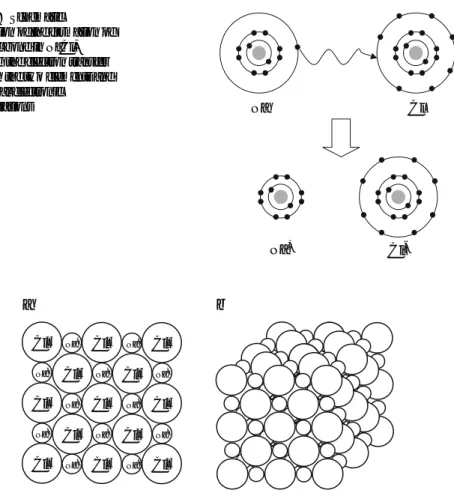
- Ionic Bonds
- Covalent Bonds
- Mixed Bonds
- Metallic Bonds
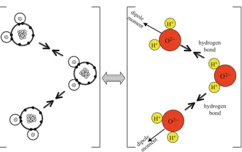
- Secondary Bonds
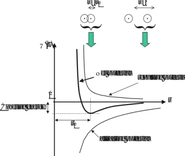
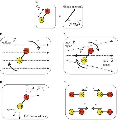
The attractive part of Figure 1.7 can be estimated from the sum of the Coulomb potential energies between the ions (see Problem 11). A van der Waals bond results from the attraction caused by the current dipole of one atom inducing a dipole in another atom.
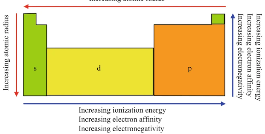
Atomic Property Trends in the Periodic Table
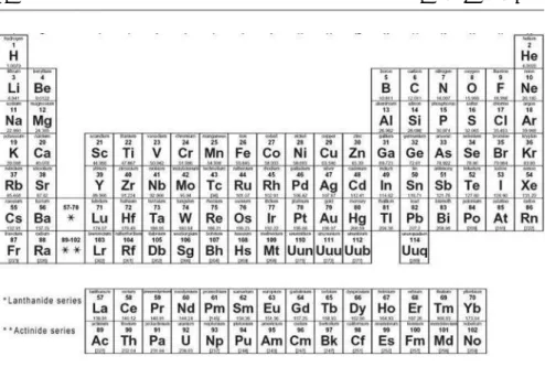
- The Periodic Table
- Atomic and Ionic Radii
- Ionization Energy
- Electron Affinity
- Electronegativity
- Summary of Trends
The electron configuration of an atom (especially its valence shell) is a primary determinant of the atom's properties. The electron affinity is the potential energy change of the atom when an electron is added to a neutral, gaseous atom to form a negative ion.
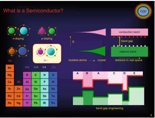
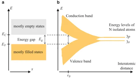
Introduction to Energy Bands
We can therefore say that, for a perfect crystal under equilibrium conditions, a plot of the allowed electron energies versus the distance along a preselected crystalline direction (x) is as shown in Fig.1.17a. When the atoms get close to each other, the energy levels change as shown in the figure, as a result of the interaction between the atoms.
Summary
Which group in the periodic table would you expect to have the greatest electron affinities. Why do none of the noble or inert gases (elements in the rightmost group) have electron affinity values listed in Appendix A.3 Fig.
Introduction: The Carbon Atom
Isotopes of Carbon Atom
What is the probability that the particle is in the second state (n¼2) of the new well immediately after the change. These locations correspond to the boundaries of the Brillouin zones defined in the previous subsection.
Electronic Con fi guration
Binding Energies
This table provides useful constants regarding covalent bonds involving the carbon atoms: the bond energy D, which can be interpreted as the energy required to break the bond, and the bond distance between the two atoms, R (Table 2.2).
Covalent Bonding Between Carbon Atoms
The carbon-carbon single bond is a sigma bond and would be formed between one hybridized orbital of each of the carbon atoms. In fact, the carbon atoms in the single bond need not be of the same hybridization.
Carbon Allotropes
In the next section, we will look at the structure of the most important allotropes of carbon currently known. Perhaps the answer is that it is the mystery of the carbon-carbon, sp, and sp2 and sp3bond. dipole-dipole coupling).

Carbon Fullerenes
Buckyballs
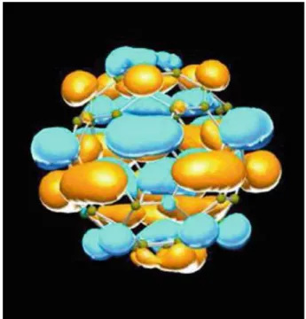
The irreducible representations of the icosahedral point group are used to determine the appropriate molecular orbital eigenfunctions. The electronic structure of the solid is composed of bands derived from the molecular orbitals of the individual goat balls.
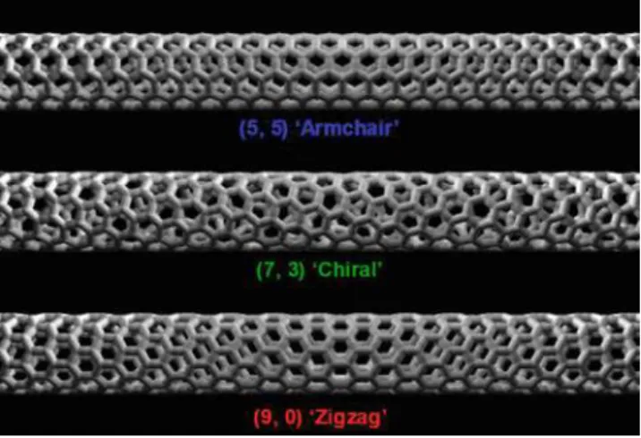
Graphene and Nanotubes
Thus, the two atoms are symmetrical and the energy level of the bound electron is the same. In this case, the states of the system described by the wave function Ψ(x,y,z,t) are called stationary states and the total energy of the system is conserved (over time).
Definition of Bonding Energy and Energy Bands
Band Structure of Fullerenes (Buckyballs)
Band Structure of Carbon Nanotubes
Background Needed for Energy Levels and Band
Tight Binding Method
Free Electron Method
Summary
In Section 2.2 we briefly introduce the reader to the concept of coupling in periodic systems. Bloch bands also lead us to the concept of holes in the valence bands and the effective mass of electrons and holes.
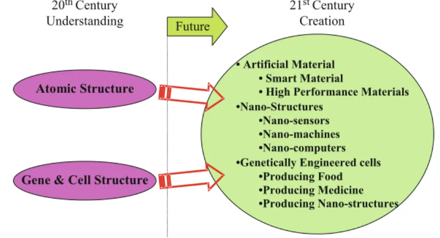
Conclusion: The Future
Here one tries to create or observe charge polarization and the pull of the polarization induced in the adjacent layers to form new electronic polarons and bipolarons. One of the mysteries of solid-state carbon physics is how far one can go with single-particle mean-field theories.
Introduction
Liquids As the temperature of a gas decreases, the kinetic energies of the molecules or atoms decrease. When the boiling point is reached (Fig. A.3 in Appendix A.3), the kinetic energy will equal the energy of attraction between molecules or atoms.
Crystal Lattices and the Seven Crystal Systems
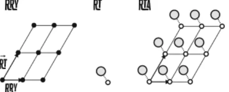
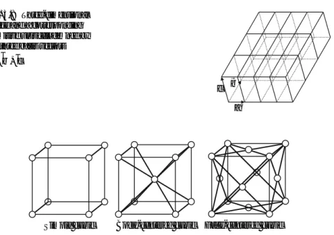
A mesh can be represented by a set of translation vectors as shown in the two-dimensional (vectors!a, !b) and three-dimensional (vectors!a, !b, !c) meshes in Fig.3.6a, c, respectively. Taking the origin at a grid point, the position of each grid point can be determined by a vector which is the integer sum of the translation vectors.
The Unit Cell Concept
A primitive unit cell is in many cases characterized by non-orthogonal lattice vectors (as in Fig. 3.8). Since one likes to visualize the geometry in orthogonal coordinates, a conventional unit cell (but not necessarily a primitive unit cell) is often used.
The Wigner-Seitz Cell
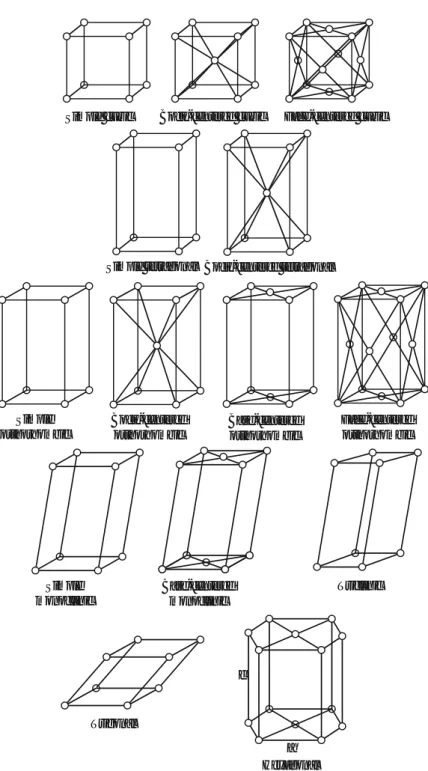
Bravais Lattices
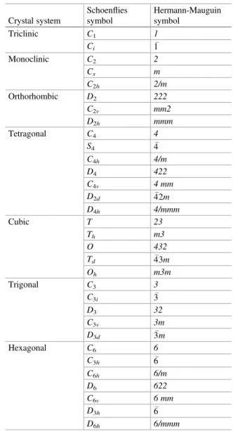
Point Groups
- C s Group (Plane Reflection)
- C n Groups (Rotation)
- C nh and C nv Groups
- D n Groups
- D nh and D nd Groups
- C i Group
- C 3i and S 4 Groups
- T Group
- T d Group
- O Group
- O h Group
- List of Crystallographic Point Groups
This point group can also be seen as a result of combining an element of the Dn group and aσh (horizontal) reflection plane. It is important to realize that the roto-inversion is a single symmetry operation, i.e. the rotation is not independent of the inversion.
Space Groups
And all symmetry operations of the group O combined with an inversion through the point centered on the body of a cube (24 elements). The previously considered point groups are constructed by considering all possible combinations of the basic symmetry operations (in-plane reflections and rotations) discussed in subsections 3.6.1 to 3.6.11.
Directions and Planes in Crystals: Miller Indices
It also follows that the grid plane with Miller indices (hkl) will be intersected by the axis!a , !b , !cat distanceNah ,Nbk ,Ncl where Ni is an integer. Miller indices for Table 3.2 List. In cubic systems such as simple cubic, body-centered cubic, and face-centered cubic lattices, the axes in Fig. 3.24 are chosen to be perpendicular, i.e. the unit vectors are chosen perpendicular and have the same length equal to the side of the cubic unit cell.
Real Crystal Structures
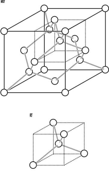
- Diamond Structure
- Zinc Blende Structure
- Sodium Chloride Structure
- Cesium Chloride Structure
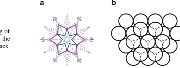
- Hexagonal Close-Packed Structure
- Wurtzite Structure
- Packing Factor
The Bravais lattice is face-centered cubic with a basis consisting of two identical atoms offset from each other by a quarter of the cubic body diagonal. The Bravais lattice is simple cubic and the basis consists of two atoms located at the corner (0,0,0) and the center position (½,½,½) of the cubic unit cell.
The Reciprocal Lattice
A Let us consider the fcc lattice shown in the figure below and an atom located at one corner of the cubic unit cell. Its nearest neighbor is an atom which is located in the center of the adjacent face of the cubic unit cell and which is at a distance of pffiffi2.
The Brillouin Zone
The concept of reciprocal or momentum space proves to be extremely important for the classification of electron states in a crystal in quantum theory.
Summary
How many lattice points are contained in the unit cell of each Bravais lattice in the cubic system. Show that the packing factor of the diamond structure is 46% of that of the fcc structure.
The Quantum Concepts
- Blackbody Radiation
- The Photoelectric Effect
- Wave-Particle Duality
- The Davisson-Germer Experiment
This potential is related to the work function Φm via qV0 ¼hcλ Φm, where λ is the wavelength of the incident photon. Lenard was then able to investigate the photoelectric effect when the frequency of incident light was varied.

Elements of Quantum Mechanics
- Basic Formalism
- General Properties of Wavefunctions
- The Time-Independent Schrödinger Equation
- The Heisenberg Uncertainty Principle
- The Dirac Notation
- The Heisenberg Equation of Motion
Now let's work with the wave function with the energy operator expressed in terms of the time derivative. In the time-independent view, the total energy operator is H_, also called the Hamiltonian of the system.

Discussion
Equation (4.31) is of great importance in theoretical physics and has no direct analogy in classical physics; it has only a formal analogue called the Poisson Bracket. 4.31) is in particular a statement that the velocity operator depends on the structure of the Hamiltonian and is not always given only (x-direction) by the operator ih1. In general, however, the system is in a superposition of eigenstates, and the result of the measurement is the weighted superposition as given by Eq.
Simple Quantum Mechanical Systems
- Free Particle
- Degeneracy
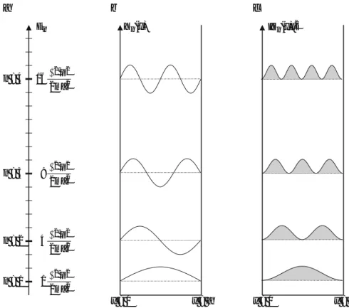
- Particle in a 1-D Box
- Particle in a Finite Potential Well
The particle in a 1-D box can be thought of as bouncing off the walls of the box and the probability of finding a particle atx in the box is shown in Fig.4.8c. The boundary conditions include the continuity of the wave function Ψ(x) and its first derivative dΨdxð Þx at points x¼0 and x¼a.
Discussion
In addition to the quantization of energy levels, there is another important quantum concept illustrated by the finite potential well: the phenomenon of tunneling. This analysis would lead to the same result as for a free particle, i.e. a continuum of energy states E > U0 is allowed.
The Harmonic Oscillator
This is called "the zero-point vibrational energy". It is also a consequence of Heisenberg's uncertainty principle, being a manifestation of the fact that when a particle is confined in space by a potential, its momentum and thus its energy can never be zero. The exact solution of the harmonic oscillator problem can be easily extended to the three-dimensional case, provided that the potential V(x,y,z) is separable and a sum of the potentials in the three spatial directions: .
The Hydrogen Atom
- Motion in a Spherically Symmetric Potential
- Angular Momentum
- The Radial Wavefunction of the Hydrogen
- The Unbound States
- The Two-Dimensional Hydrogen Atom
- The Electron Spin
Then we note that the angular momentum operators in all three directions commute with the Hamiltonian of the hydrogen atom, i.e., the operators complete: In this section we have addressed the solution of the hydrogen atom problem in quantum mechanics.

Relativity and Quantum Mechanics
The Electron Spin Operator
Now that we know where the spin of the electron comes from, we can proceed to formulate the Pauli Dirac spin operators.
The Addition of Angular Momentum
The Pauli Principle Applied to Many-Electron Systems
For example, two electron spins1 and2 can combine to form S¼s1+s2 with possible total spin statesS¼1 and S¼0.
Summary
When we use Slater's determinants instead of a simple product of wave functions, we incorporate the fact that although electrons in this order do not strictly interact, there is an implicit correlation in their spatial distribution caused by the Pauli principle. The spin quantum number brilliantly follows the Dirac equation, or a linearized form of the Klein-Gordon equation, which is a manifestation of the fact that the "empty vacuum" is only a time-averaged concept.
The Electron in a Magnetic Field
Degeneracy of the Landau Levels
To count the degeneracy, it is convenient to assume that the system is in a cubic box of size L with periodic boundary conditions such that Ψ(x+L,y+L,z+L)=Ψ(x,y,z). The transition from the two-dimensional Bz = 0 spectrum to the discrete and gL-fold degenerate Landau spectrum is shown in Fig. 4.15.
Discussion
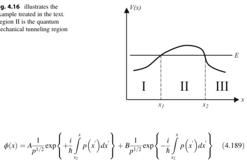
The Wentzel Kramer Brillouin Approximation
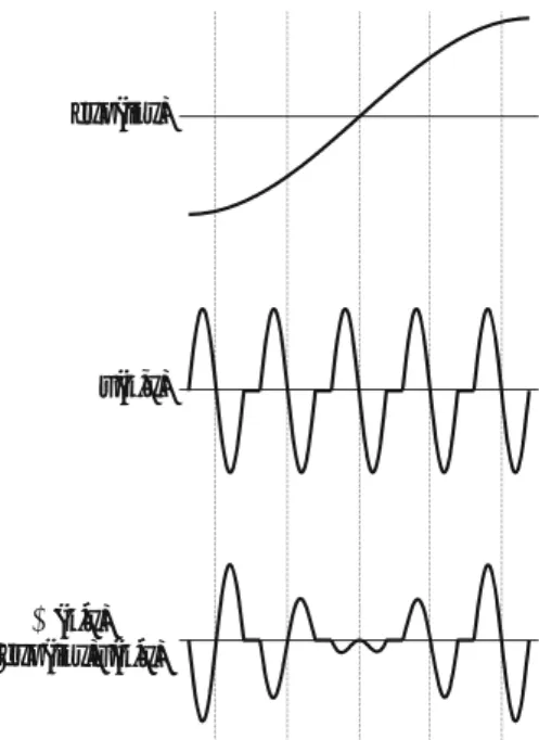
To obtain the full solutions, one connects the different regions defined above by requiring the continuity of the wave function and its derivative. In region I, between 0 and x1, the energy E is greater than V(x), sop(x) is real, phase oscillating, and the wave function is of the form Eq.
Quantum Mechanical Perturbation Theory
Time-Independent Perturbation
It is therefore very important to be able to include the effect of such new interactions, at least to some extent, and study what they do to the wavefunctions and energy levels of the system. We consider the initial Hamiltonian H0, for which we assume that we have normalized eigenfunctions Φn and energy levels En.
Nondegenerate Perturbation Theory
With a wave function given in the first order by:. while previously the matrix element of the potential is defined by: . It is interesting to note that the second-order term for the ground state energy is always a term for lowering energy, regardless of the nature of the perturbation.
Degenerate-State Perturbation Theory
Knowing the unperturbed wave functions and energy levels, we can calculate the perturbed ones. 4.205), while simple, are some of the most useful results of quantum mechanics. The quadratic has two different roots, and the degeneracy of the ground state is now canceled out by the perturbation.
Final Summary
If the energy is interpreted as the kinetic energy of the electron, what is the corresponding speed of the electron. How the field affects the symmetry of the charge distribution in the ground state.
Introduction
Electrons in a Crystal
- Bloch Theorem
- One-Dimensional Kronig-Penney Model
- Energy Bands
- Nearly Free Electron Approximation
- Tight-Binding Approximation
- Dynamics of Electrons in a Crystal
- Fermi Energy
- Electron Distribution Function
The energy difference between branches at points A1 and B1 (A2 and B2) is the energy gap that arises as a result of the periodic potential in the grid. A negative effective mass means that the acceleration of the electron is in the direction opposite to the external force exerted on it, as shown in Eq.
Density of States (3D)
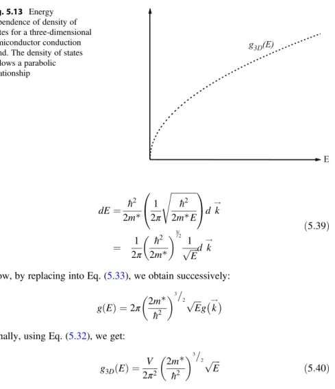
Direct Calculation
Q Calculate the ink-space density of states for a cubic crystal with a side of only 1 mm. For a bulk semiconductor crystal, the electron density of states is calculated near the bottom of the conduction band, because this is where the electrons that cause the most important physical properties are located.
Other Approach
Electrons and Holes
Band Structures in Real Semiconductors
First Brillouin Zone of an fcc Lattice
First Brillouin Zone of a bcc Lattice
First Brillouin Zones of a Few Semiconductors
Two-Dimensional Semiconductors and Transition Metal
Examples: Graphene (G) and TMDC
Graphene Band Structure: Nearest Neighbor
Two-Dimensional Metal-Dichalcogenide
Example: Fabrication of Flexible Transistors
Summary: Discussion
Band Structures in Metals
The Kane Effective Mass Method
The Effect of the Spin-Orbit Coupling
Summary
Phonons and Thermal Properties
Introduction
Interaction of Atoms in Crystals
One-Dimensional Monatomic Harmonic Crystal
One-Dimensional Diatomic Harmonic Crystal
Extension to Three-Dimensional Case
Phonons
Sound Velocity
Summary
Thermal Properties of Crystals
Introduction
Phonon Density of States (Debye Model)
Thermal Expansion
Thermal Conductivity
Summary
Problems for Thermal Properties of Crystals
Introduction
Density of States
Effective Density of States (Conduction Band)
Effective Density of States (Valence Band)
Mass Action Law
Doping: Intrinsic Versus Extrinsic Semiconductor
Charge Neutrality
Fermi Energy as a Function of Temperature
Carrier Concentration in an n-Type Semiconductor
Summary
Introduction
Electrical Conductivity
Ohm ’ s Law in Solids
The Case of Semiconductors