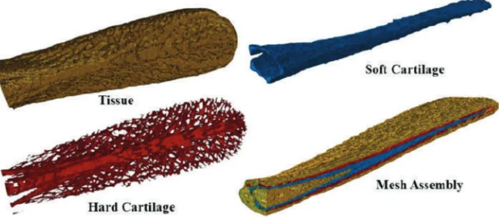
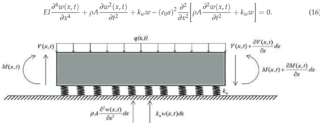
A diagram of the load condition on a simply supported concrete beam is shown in Figure 5. A cross section of the mesh assembly shows the location of the three rostrum components in the actual model.

Results
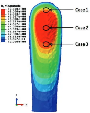
Figure 15a shows the maximum principal stresses on the upper surface of the soft cartilage part of the rostrum. Figure 17a shows the maximum principal stresses on the upper surface of the hard cartilage portion of the rostrum.
Conclusions
Comments on the Transdisciplinary Approach
In Proceedings of the European Conference on Constitutive Models for Rubber, Paris, France, 4–7 September 2007. Medium-scale modeling of the effect of size on the fracture process zone of concrete.
Nonlocal FEM Formulation for Vibration Analysis of Nanowires on Elastic Matrix with Different Materials
- Introduction
- Euler–Bernoulli Nanobeam Resting on a Winkler Elastic Foundation The nonlocal stress tensor σ ij at point x is expressed as follows [14]
- Solution to the Vibration Problem
- Results and Discussion
- Conclusions
To obtain the weak form of the governing equation of the Euler-Bernoulli nanobeam resting on a Winkler elastic basis, the residue can be expressed as:. The effects of temperature rise and Winkler parameter on the first three natural frequencies of the nanowires are revealed in Table 8 .
Trustworthiness in Modeling Unreinforced and Reinforced T-Joints with Finite Elements
Previous Researches
However, for an exhaustive description of the tests, the reader is invited to the articles [4,5]. The present section illustrates the details of the numerical simulations performed with 3-D solid elements in reference [5].
Present Modeling
At the same time, two phases of joint behavior can be subtracted, such as the linear phase and the plastic phase. In conclusion, all the results obtained from these two papers will be used in the fundamental FE model calibration step of this work. During the development of the contact between the tendon and the reinforcement made for reinforced T-joints, the contact mechanical properties are imposed by fixing the relevant points such as tangential and normal behavior in the regularity of the contact interaction.
For the sake of further comparison, the deformed shape at the center of the joint will be considered. The density of the coarse and medium mesh is obtained by setting a unique size to the T-joint instance. For the final view of the instance in the case of the item mesh, please consider Figure 3d.
![Table 4. Values of E and ν of preliminary simulations [17].](https://thumb-ap.123doks.com/thumbv2/1libvncom/9200819.0/40.723.101.616.220.318/table-values-e-ν-preliminary-simulations.webp)
Results
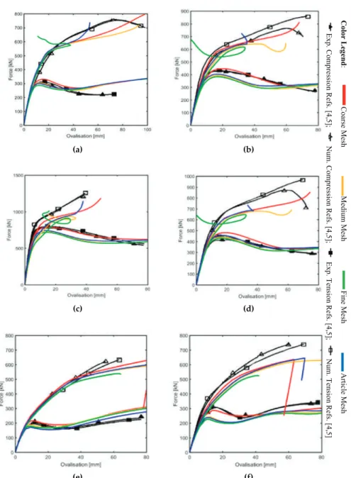
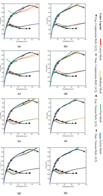
In the case of the EX-06, it is the one that lags the most from the references, but with the S8R element type the differences are reduced. In addition, in this first improvement, for the EX-08 specimen using the S8R element, the ovalization direction change is also avoided in the fine mesh. Therefore, some gaps can be seen in the presentation of the rings as far as reference [4,5] is concerned.
Figure 12a,b shows the overall picture of the unreinforced specimens of the Experimental Case (EC) (reference figures from [4,5]) and the Research Case (RC) (the current simulations). The separation of the outer surface of the chord from the double plate (which perfectly matches the chord in its original shape) can be observed. Figure 14a-c illustrates the separation of the doubling plate from the chord at the intersection between the brace and the doubler.
Summary and Conclusions
An almost 40% improvement was obtained for β=0.54 than the experimental case, but a smaller value was found for β=0.28, where the research value is five percent less than the experimental one, which is sixteen percent. Therefore, it can be said that the two types of reinforcement have the ability to distribute the axial load of the beam over a larger area of the chord, with a consequent improvement in terms of increased strength. By using shell elements instead of more expensive (in terms of computational costs) massive elements, the problem of contact and the introduction of element thickness is solved.
Missing data in the reference papers inevitably led to some differences in the results, which are partially resolved by using a different true stress-strain relationship. However, due to the good agreement between research and experimental results, the former can be developed with parametric studies to extend the above considerations to different types of conclusions. In addition, this research can be considered in studies involving composite materials as a reinforcing phase for damaged or weak joints.
Future Developments
The effects of chord length and boundary conditions on the static strength of a tubular T-joint under stirrup compression loading.Mar. Capacity of steel CHS X-joints reinforced with external stiffening rings in compression. Thin-walled construction. Experimental, theoretical and numerical analysis of K compound made from CHS aluminum profiles. Thin-walled construction.
Experimental Study and Theoretical Analysis on the Ultimate Strength of High Strength Steel Tubular K Connections. Thin-walled structure. Behavior of Inserted Stainless Steel Tubular X-Connectors with CHS Chord under Axial Compression. Thin-walled structure. Fatigue behavior and design of welded tubular T-joints with CHS strut and concrete-filled chord. Thin-walled structure.
A Complex Variable Solution for Lining Stress and Deformation in a Non-Circular Deep Tunnel II
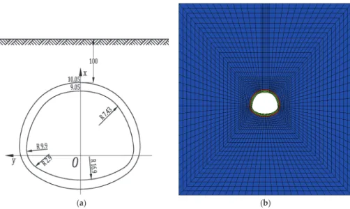
Problem Statement and General Consideration
It is assumed that the region S1 in the z-plane can be conformally mapped onto a ring (O1) in the ζ-plane. The surrounding rock, region S2 in the z-plane, can be conformally mapped to region O2, which is the area outside the outline L2 in the ζ-plane, see Figure 1. In most situations it is accurate enough to take only the first few of the Jkof series. θandρ are assumed to be two polar coordinates of point ζ in the ζ-plane.
In the complex variable method, the solution is expressed in terms of two functions ϕ and ψ, which are to be analyzed in the area S1 occupied by the elastic material. The expressions Γw(ζ) and Γw(ζ) should not be included in continuity equation (16), as they define the initial soil stress and deformation in the surrounding rock when tunnels are excavated. Equations (16) and (17) relate to the continuity of deformation and the stress field across the liner-rock interface due to the anti-slip condition.
Solution
Stress functions ϕ1(ζ),ψ1(ζ),ϕ2(ζ)andψ2(ζ) should satisfy the continuity boundary conditions on R2 circles and satisfy the boundary conditions on R1 circles. It can be concluded as: where fR21 and fR22 are displacement components of boundary R2 in the liner and rock respectively. To obtain a solution to equations, Li's method must be introduced, which converts the form of the multiplication of two infinite polynomials into an infinite matrix, which can be easily calculated and interpolated by a computer.
The coefficients ak, bk, ck, dk, hka and mkre, which are required in the final stress function, are obtained by equation (37). Since the coefficients h∞ and m∞ are known, the number of unknown coefficients in the set of equations is reduced from (6k+4) to (6k+2). The number of unknown coefficients is equal to the boundary conditions in which all coefficients are determined uniquely.
Implementation
Since the coordinates of the analytical solution and the numerical simulation are different, it is necessary to rewrite the results. The comparison of the rewritten results between the analytical solution and numerical simulation is shown below. Figure 5 shows the radial displacement of the tunnel along the rock-lining interface predicted by the analytical solution.
The radial displacement of the tunnel along the periphery of the inner liner is illustrated in Figure 6, which shows that the radial displacement of the analytical solution and the numerical simulation are all zero at α=75◦. The voltage value curves showed that the new analytical solution and the numerical simulation were in reasonable agreement. The normal and shear stress values of the tunnel along the periphery of the inner liner were close to zero, proving the high accuracy.
4D Remeshing Using a Space-Time Finite Element Method for Elastodynamics Problems
- Principle of the Method
- Numerical Analysis
- Numerical Results on Mesh Adaptation
- Conclusions
For that purpose, as in the cases of the discontinuous Galerkin method [2,10,11] and the LArge Time Increment (LATYN) method [1,12], the variational formulation is written on the entire space-time domainΩ×[0,T]. 16] also proposed a progressive mesh generation, in the context of the discontinuous Galerkin method. Preliminary results on the stability of the method were established in [22] and compared with the Newmark integration scheme.
For 1D space-time elastodynamic applications, using the STFEM method with linear simplex elements is similar to using the implicit Newmark integration scheme with δ=1/2 and θ=1/3. Size of the time step of discretization required for stability with respect to the average size of the 3D finite elements. The results of the presented calculations are obtained for space-time plates of 10−7s (this corresponds to using a time step equal to 10−7s).

Integration of Direction Fields with Standard Options in Finite Element Programs
The Integration of Direction Fields by Means of the Orthotropic Heat Equation
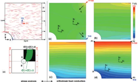
Consistent with the hypothesis in the previous section, it will be shown that orthotropic heat conduction can be used for the integration of this equation. The heat conduction equation (4) is solved in the FE programs. 7) The solution T(x,y) of equation (7) can be visualized by isotherms, representing a directional field yT´. Whether the orthotropic heat conduction problem in Equation (11) is solved, which is not generally available as a computational option in FE programs, or Equation (7) is solved through an FE program, the same isotherms result and tangent to the given direction field = f(x,y).
Relationship between the isotherms of extremely orthotropic heat conduction and the characteristics of a first-order partial linear differential equation. This is achieved with an orthotropic heat conduction analysis that specifies a linear temperature distribution fory > 0 along the right boundary (Figure 5a). In Section 2.2 it was shown that the Fourier heat conduction equation (11) can be traced back to the general linear differential equation (12).
Procedure and Application Examples
The integration of the corresponding characteristic equation (13) yields characteristics identical to the isotherms in the Fourier heat conduction equation (11). The theory of characteristics also includes the treatment of boundary conditions [14], the rules of which can be fully applied to the Fourier heat conduction equation (14). The PS direction field from the structural calculation is adopted as material orientation for the thermal conductivity in the thermal analysis.
The influence of the temperature boundary condition with two nodes at points P2 and P3 (Figure 7d) on the course of isotherms is no longer observable fork1/k2 > 104. The isoclines result from equation (16), i.e. the contour lines of the stress expression on the right should be visualized; see also figure 2c. Repeating the thermal conductivity analysis with a three-node temperature boundary condition (P0:T= 0◦C, P1:T= 1◦C, P2:T= 2◦C, Figure 10b) improves the uniformity of the isotherms.
Discussion and Conclusions
The integration of the stress components [σxxσyy σxy] over the thickness produces normal forces N=[NxxNyyNxy] and bending moments M=[MxxMyyMxy]. It makes sense to place the M layers on the inside and outside and the N layers in the middle of the shell. When evaluating a TFP laminate, one is faced with the variable fiber volume fraction due to the divergent and convergent streamlined nature of the fiber layer.
Showing the gradient of the temperature field is identical to showing the isotropic heat flux,q=k·degree(T) withk=k1=k2. Assuming that the trajectory of the isotherms (paths) is to be used for fiber placement in FRP structures, the visualized isotherms must be converted to polylines with x, y, and z coordinates. In Proceedings of the 8th Eurographics Workshop on Visualization in Scientific Computing, Boulogne-sur-Mer, France, 28-30. April 1997;.