Numerical Simulation

The first section of the book presents models and simulations for analyzing the behavior. The third section of the book presents various problems of heat transfer involving fluids.

Models and Applications in Medicine

In Chapter 15, Ketabdari discusses and evaluates different free surface simulation methods based on a computational grid. As the editor of this book, I would like to thank all the authors who contributed to this book, as well as the reviewers for their rating.

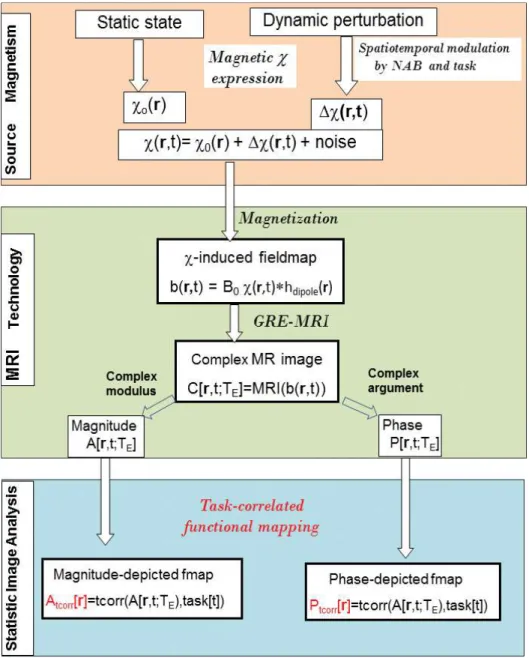
BOLD fMRI Simulation

Introduction

Brain functional imaging based on MRI and the endogenous BOLD contrast is called BOLD fMRI. Nevertheless, only the MR size image has been exploited for brain imaging (structural or functional).

Models and methods

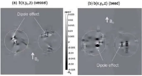
Definition of 3D vasculature and magnetic susceptibility source (χ)
Calculation of χ-induced fieldmap
Multivoxel partition of VOI
Calculation of intravoxel dephasing signals (Monte Carlo method)
Intravascular (IV) and extravascular (EV) signal separation
Diffusion effect
Volumetric BOLD fMRI simulation

It is straightforward to implement 4D BOLD fMRI simulation based on the repetition of volumetric BOLD fMRI simulations for each snapshot recording over a BOLD activity. The 4D BOLD fMRI simulation involves a predefined 4D source χ[r,t] and two output 4D images (A[r,t] for magnitude and P[r,t] for phase, as defined in Eq.

Figure 1. A BOLD fMRI model consists of three stages. The stage of “Source Magnetism” provides a dynamic magnetic susceptibility source for the stage of “MRI Technology”

Simulation results

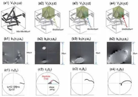
Single voxel signal simulations
Volumetric BOLD fMRI simulations

Numerical simulations of 4D BOLD fMRI data acquisition. a1, a2) BOLD magnitude images captured in an ON and OFF state and (a3) the magnitude signal time courses on two voxels (marked by x and o(a1, a2), extracted from the 4D magnitude dataset A[r, t]). b1, b2, b3) for the BOLD phase images in P[r,t] and the voxel phase time courses. Numerical simulations of 4D BOLD fMRI data acquisition. a1, a2) BOLD magnitude images captured in an ON and OFF state and (a3) the magnitude signal time courses on two voxels (marked by x and o(a1, a2), extracted from the 4D magnitude dataset A[r, t]).

Figure 8. Multiresolution complex-valued voxel signals due to voxel subdivision. As the voxel size is dyadically re‐

Discussion

Nevertheless, our 4D BOLD fMRI simulations also show that image noise has a strong effect on the fmap obtained from an image magnitude or phase dataset, due to a simplified spatiotemporal modulation model for numerical BOLD χ terms. Data acquisition with BOLD fMRI is not analytically feasible due to the involvement of diverse parameters.

Conclusion

The numerical simulation on 4D BOLD fMRI for task-evoked functional mapping shows that the extraction of functional activity by a task correlation technique is sensitive to data noise. The finding in source-image mismatch inspires us to search for the underlying magnetic source of BOLD fMRI for more accurate brain functional mapping.

Author details

Both the MR magnitude and the phase images differ spatially from the predetermined magnetic susceptibility distribution. Overall, the numerical simulations on BOLD fMRI allow us to explore the insights of a single-voxel signal, a multivoxel image and a video of brain functional BOLD activity with respect to various parameter settings.

Calhoun, “Volumetric BOLD fMRI Simulation: From Neurovascular Coupling to Multivoxel Imaging,” BMC Medical Imaging, vol. Calhoun, "Understanding the Morphological Mismatch between Magnetic Susceptibility Source and T2* Image", Magnetic Resonance Insights, vol.

Basics of Multibody Systems: Presented by Practical Simulation Examples of Spine Models

Basics of model building and simulation

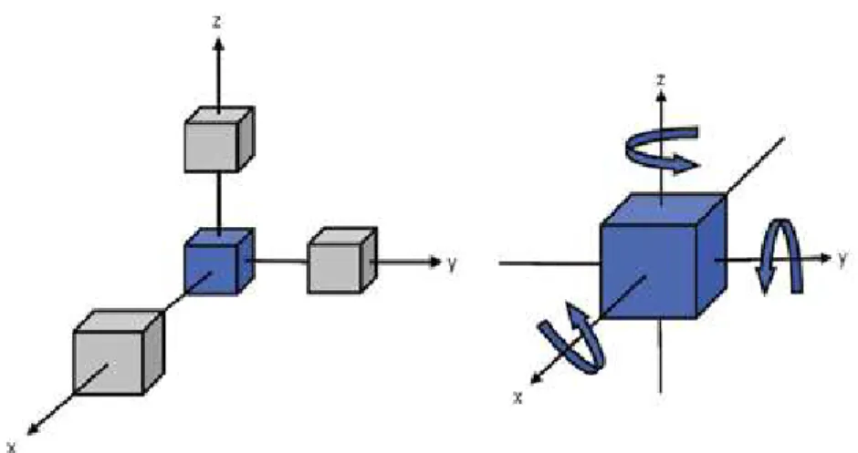
According to [19], the DoF of a model is determined by a number of independent state variables that characterize the movement of the body. Furthermore, the motion of the MBS system depends on the inertial properties of its bodies, masses, inertia tensors, and its centroids.

Figure 1. Different elements of polygon mesh modeling.

MBS lumbar spine models

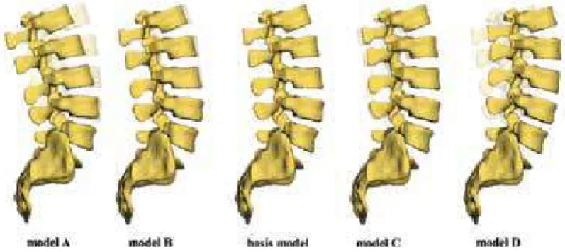
Structure of the spine model
Surface generation
Modeling of the biomechanical behavior of the spinal structures
Validation and sensitivity analysis of the model

It should be noted that a detailed modeling of the facet surfaces is accompanied by a large. A comparison of the different spine models with the corresponding muscle models is performed (see section 4).

Figure 3. Surface generation through segmentation (left) and visualization (right) plugins [29].

Practical application examples of simulation

Effects of different spine alignments in the standing position
Effects of overweight on the spinal biomechanics
Application possibilities of biomechanical computer models in medicine

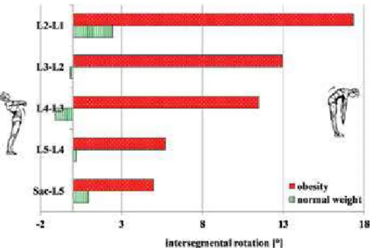
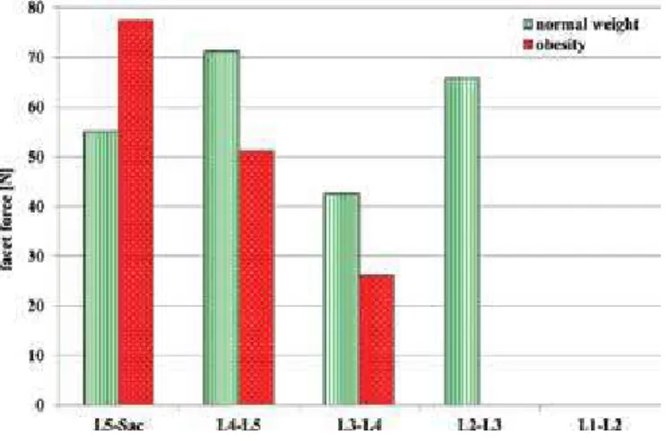
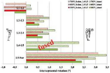
In the case of a person of normal weight, in general the intervertebral deformities in all FSUs are very small (Figure 6). Increased body weight has a direct impact on the load structure of the intervertebral discs.

Figure 4. MBS lumbar spine models with different alignments: The model located in the middle has to be understood as a basic model concerning the anthropometrical and biomechanical properties for the further models A, B, C, and D.

Meaningfulness and limitation of MBS modeling

18] Juchem S: Development of a computer model of the lumbar spine for the determination of mechanical loads [dissertation]. Biomechanical MBS modeling of the lumbar spine loading situation with different body weights.

Simulation of Neural Behavior

Neuron model with a low-pass filter property

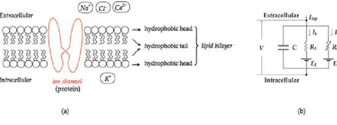
Electrical circuit model of the cell membrane
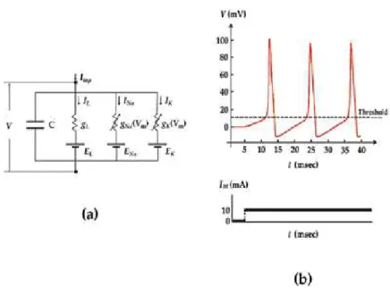
Generation of action potentials (Hodgkin-Huxley model)

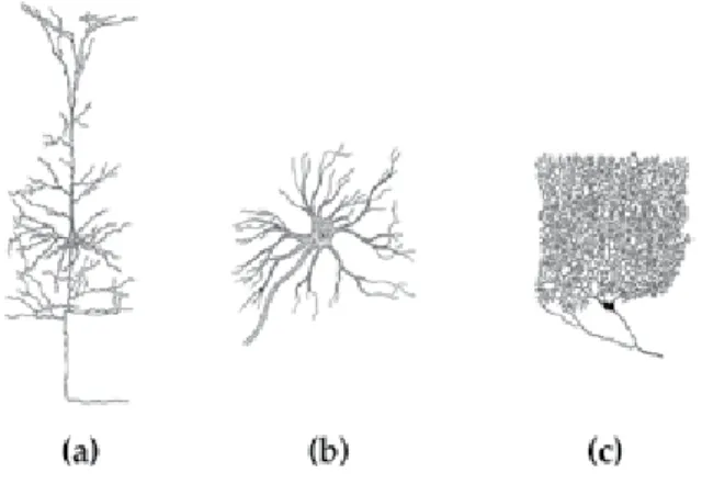
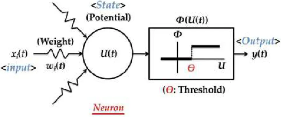
As shown in Figure 3(a), it is composed of two layers of phospholipid molecules, each of which has a hydrophilic head (circle) and a hydrophobic tail (two wavy lines), and both hydrophobic tails face each other inside the cell membrane. In this section, we provide a model that can generate an action potential, which is the basic function of a neuron. The most prominent example is the application to the perceptron, which was known as one of the powerful tools for some forms of pattern recognition.

Figure 1. Various types of neurons. (a) Pyramidal neuron (cortex), (b) motor neuron (spinal cord),and (c) Purkinje cell (cerebellum).

Neuron model with a band-pass filter property

Subthreshold resonance phenomenon
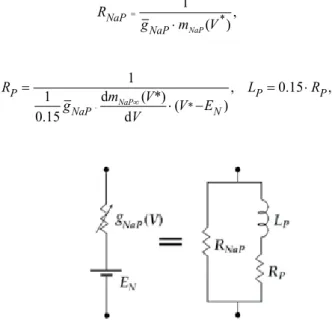
Inductive property of voltage-dependent ion channels
Properties of voltage responses to oscillatory current inputs

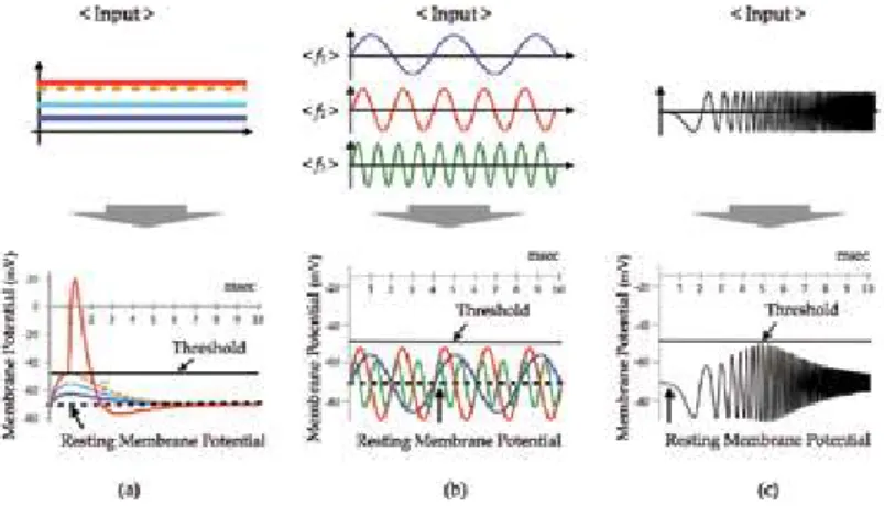
When the membrane potential V(t) changes from V* to V* + δV(t), where δV(t) is a small variation of the membrane potential from V*, the current Ih(t) also changes from Ih* to Ih*+δIh*(t), where δIh(t) is a small variation of h current caused by δV(t). When the membrane potential V(t) changes from V* to V* + δV(t), the current INaP (t) also changes from INaP* to INaP* +δINaP(t), where δINaP(t) is a small variation of NaP current caused by δV(t). In this case, no action potentials are generated because the membrane potential cannot exceed the threshold at all.

Figure 6. Subthreshold resonance phenomena. (a) DC inputs with different amplitudes, (b) AC inputs with different frequencies, and (c) a chirp current input whose frequency increases as time increases.

Conclusion

In the case of Figure 16(c), for an input frequency of 30 Hz, no action potentials are generated because the membrane potential is below the threshold value. By comparing Figure 16(b) and (d), it is clarified that the more peaks are observed than in the case of no DC bias current being input. Since no action potential is generated in the case of id= 0 μA/cm2, this is also caused by the effect of a DC bias current input.

Acknowledgements

Thus, the maximum amplitude of membrane potentials exceeds the threshold by the action of the subthreshold resonance property. On the other hand, if a DC bias current input increases to 1μA/cm2, as Figure 16(d) shows, more action potentials are generated for 13 Hz input frequency input than the case of no DC bias input. However, from the fact that many neurons in different areas of the brain have bandpass properties, a neuron should be modeled by an RLC circuit.

Numerical Simulations of Dynamics Behaviour of the Action Potential of the Human Heart's Conduction

Modelling techniques

Van der Pol model

In the considered model (5), the problem is adjusting the position of the stationary states in the phase space. It is for better frequency regulation. one of the most important existing mathematical models of the action potential. In the considered model (5), the problem is adjusting the position of the stationary states in the phase space.

Construction and analysis of proposed models

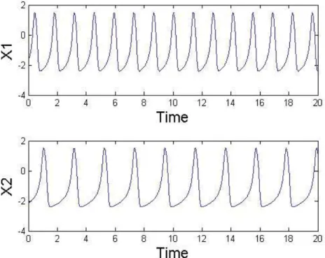
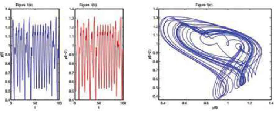
Even with this variant, we observe a shortening (as in Figure 5) of the oscillation period. The impact of the pulse is considered as the occurrence of an auxiliary current in the system. The numerical solution of the feedback system (k=1,T=0.5) excited by a rectangular pulse is shown in Figure 6.

Figure 1. Time series for reference model without feedback and delay, see Eq. (5).

Conclusions

Correspondingly large coefficient can cause synchronization, but often set points are not the values of the physiological range. In this work, by using the proposed models, we were able to reproduce the main physiological characteristics of the discussed pathologies. A simple model of the right atrium of the human heart with the sinoatrial and atrioventricular nodes included.

Mathematical and Numerical Methods

Numerical Simulation Using Artificial Neural Network on Fractional Differential Equations

Definitions and preliminaries

The Riemann-Liouville, Grünwald-Letnikov, and Caputo definitions of fractional derivatives of order α>0 are most often used among some definitions of fractional derivatives and integrals, but in this chapter, the Caputo definition will be used to work out the fractional derivative in a later procedure. Definitions of commonly used partial differential operators are discussed in the study of Sontakke and Shaikh [26].

The Riemann-Liouville fractional derivative operator can be defined as follows

The definition of fractional differential operator was introduced by Caputo in late 1960s that can be defined as follows [27]

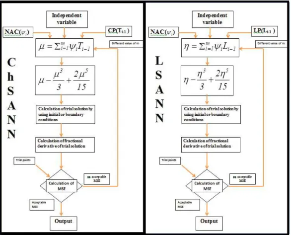
ChSANN and LSANN

Methodology
Implementation on fractional Riccati differential equation

Results and discussion

In this section, ChSANN and LSANN are applied to a fractional Riccati differential equation of the type:. The mean squared error (MSE) of equation 1) will be calculated from the following: while here as n can be defined as the number of trial points. The proposed methods gave an excellent numerical approximation of the Riccati differential equation of fractional order.

Figure 1. Model diagram of ChSANN and LSANN.

Numerical Simulations of Some Real-Life Problems Governed by ODEs

Numerical simulations for VOFHHM of neuronal excitation

Introduction
VOFHHM
Discretizations of the model using NSFD method
Numerical experiments

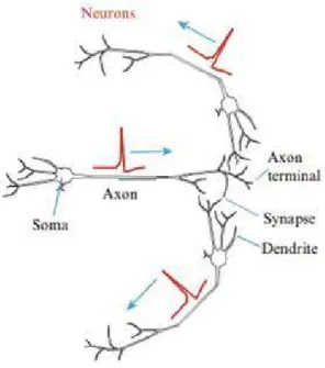
The IL current is the efflux current and indicates all currents remaining across a cell membrane except Na+ and K+ currents. HHM can be considered as one of the most successful mathematical models in the quantitative description of biological phenomena, and it is the method that can be used in deriving a squid model that is directly applicable to many types of neurons and other excitable cells [5-7]. A soma is the main body of the neuron from which extends a long cable called an axon.

Real-life models governed by nonlinear delay differential equations (DDEs)

Introduction
ABM method for the VOFDDEs
Numerical examples
The four-year life cycle of a population of lemmings model
The enzyme kinetics with an inhibitor molecule model
The Chen system model

In [27] Tavernini solved a model of the 4-year life cycle of a population of lemmings in an integer sequence. Consider the variable-order version of the four-year life cycle of a population of lemmings. In some cases, the phase portrait is observed to be stretched as the order of the derivative is reduced.

Figure 11. The numerical behavior of system (29) and chaotic attractors at α = 1.

A Multi-Domain Spectral Collocation Approach for Solving Lane-Emden Type Equations

A multi-domain pseudospectral relaxation method

The solution procedure assumes that the solution in each subinterval Λk, denoted by y(k)(x), can be approximated by a Lagrangian interpolation polynomial of the form . The solution method seeks to solve each of the system of first-order ODEs independently in each kth sub-interval Λk using the solutions obtained in the previous interval Λk−1 as initial conditions. The value of the solution at the last node y(1)(x1) is used as the initial condition when a solution is sought in the second subinterval Λ2.

Numerical experiments

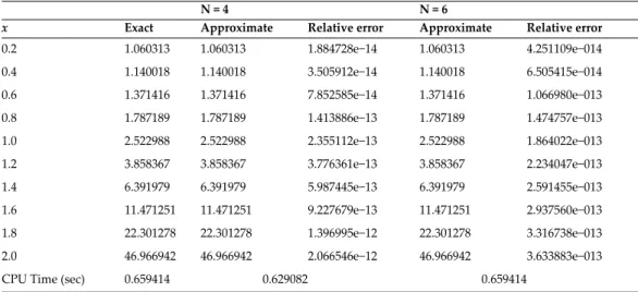
The matching between the exact and approximate solutions in Table 2 and Figures 3 and 4 validates the accuracy and computational efficiency of the multidomain pseudospectral relaxation method of Eq. The matching between the exact and approximate solutions in Table 3 and Figures 5 and 6 validates the accuracy and computational efficiency of the multidomain pseudospectral relaxation method of Eq. The superposition of the approximate solution on the exact solution implies that the multi-domain pseudospec‐.

Table 1. Analytical, approximate solutions and relative errors for Example 1.

Numerical Solution of System of Fractional Differential Equations in Imprecise Environment

Basic descriptions

Fuzzy numbers
Fuzzy-valued Function and its fractional derivative
System of fractional order fuzzy differential equations

Any interval-valued function is said to be a fuzzy-valued function if it is defined as . By the existence of limit and continuity of , the fuzzy-valued function (t) is said to be differentiable at each t0∈ a,b, if it exists, such that. In particular, modeling of differential equations of the fractional order in imprecise characteristics is achieved by including functions with fuzzy value.

Grünwald‐Letnikov’s fractional derivative

Lemma
Theorem: truncation error

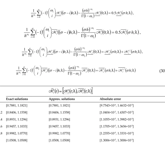
And as previously mentioned, they are taken as the fuzzy Caputo-type fractional differential operators and interpreted numerically using the Grünwald-Letnikov fractional derivative definition. Now let be a fuzzy-valued function such that , so that the Grünwald-Letnikov fractional derivative of (t) is expressed as:. Assume the nth equation of the system (19) and using Grünwald‐Letnikov's fractional derivative, we have, . or it can be rearranged as:.

Numerical illustrations

Example 1
Example 2

Following the algorithm demonstrated in Section 3, numerical experiments of several systems of fuzzy fractional differential equations are presented here. In this chapter, the system of fractional differential equations with fuzzy-valued functions was constructed to study the system in an imprecise environment. Generalizations of the differentiability of fuzzy-valued functions with applications to fuzzy differential equations.