He has developed optical coherence tomography systems to support various medical and industrial 3D imaging applications. The image penetration depth of an optical coherence tomography (OCT) system is limited by the dynamic range of the system.
Introduction
For example, one method is based on a two-channel detection technique to increase the dynamic range by reconstructing saturated signals due to the strong reflection of the sample surface. The detected signal was split into two channels with the ratio of signal levels precisely calibrated.
Correction of saturation effects
The schematic diagram of the SSOCT system for correction of saturation effects is shown in Figure 1 [11]. The division ratio of the power divider is accurately calibrated using a high-performance oscilloscope.
Compensation of signal attenuation
Shadow removal and contrast enhancement in optical coherence tomography images of the human optic nerve head. We report that high lateral resolution and optical coherence tomography (OCT) with high image quality can be achieved using a multi-frame super-resolution technique.
OCT system and superresolution principle 1 SD-OCT and lateral resolution limit
- Improving lateral resolution by high density scanning
- Improving lateral resolution by the multi-frame superresolution for in vitro imaging
- Estimating the unknown shifts to improve lateral resolution by multi-frame superresolution for in vivo imaging
- SD-OCT image acquisition and superresolution processing
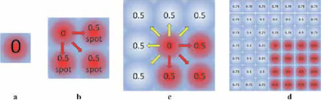
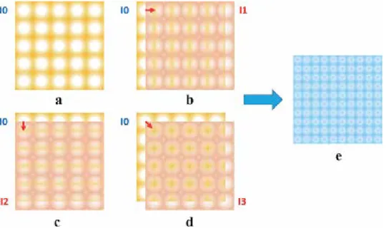
The illustration shows our superresolution reconstructed image from multiple low-resolution frames with subpixel shifts. a) The first image of the x-y plane I0 with 55 pixels is set as position 0, as a reference. We treat x as a random variable over the coordinate locations in u and v . The best transformationT can be estimated by algorithms [64–66] to maximize the mutual information I between u and v . KyT is considered as the movement operator F^ kin equation 4) to translate the side image with low resolution in vivo to the reference one.
Experiments and results
Lateral resolution, image quality, and efficiency improvement
The resolution (the space between two lines, the same as the width of 1 line) of groups 4-7 is given in Table 2. a) The image of groups 4-7 of the negative 1951 USAF test target was taken by the ZEISS SteREO Discovery. V20 microscope. Compared with Figures 10(B)–(E) , the results in Figure 11 clearly show the advantage of our multi-frame super-resolution processing with less scanning time.
Improved lateral resolution imaging of microstructure samples
So far, we have successfully demonstrated the effective lateral resolution and image quality enhancement by the multi-frame super-resolution processing with low-resolution offset C-scans. As our previous report, the multi-frame super-resolution processing can improve the lateral resolution of our SD-OCT with a 19mm focal length lens by three times, reaching 1–2 μm [37].
Improved lateral resolution imaging of in vivo 3D fingerprint The previous section has successfully demonstrated the superresolution
However, due to low resolution, the SVP image of the original rare C-scan could not clearly show the distribution of eccrine sweat glands. We observe only the outer pattern of the fingerprints, but with very blurred images of the eccrine sweat glands and the internal structures of the fingerprints.
Conclusion
Improving lateral resolution and image quality of optical coherence tomography by the multi-frame superresolution technique for 3D tissue imaging. Adaptive-optics optical coherence tomography for high-resolution and high-speed 3D retinal in vivo imaging.
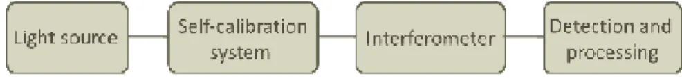
Description of the measurement scheme
- Laser system
- Calibration of the laser emission
- Fiber-optic interferometric system .1 Michelson interferometer
- Detection and processing
One of the beams is directed at the reference surface (mirror) and the other at the sample. From this last expression, it is possible to determine the thickness of the studied sample.
Measurements with the OCT system
Long-distance measurements
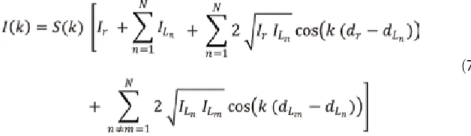
It is clear that the amplitude depends on the spectral profile of the light source (S(k)) and it is desirable to eliminate this dependence. The decrease in the visibility of the processed signal can be observed in Figure 11 where, as
Measurement of multilayer transparent samples
P1,4¼T1ngþT3þT2ng (27) From these equations it is possible to obtain the dimensions of the container as. The latter is schematized in Figure 14, where the thicknesses of the different layers (Giand Ai) are indicated, as well as the intensities that are reflected in the different interfaces (Ii).
Measurement of opaque objects
Conclusions
Fourier domain mode locking (FDML): A new laser operation regime and applications to optical coherence tomography. Non-clinical uses of optical coherence tomography (OCT) have been mainly in the non-destructive testing of materials on an industrial scale and for the study of priceless historical artifacts [1].
Full-field TD-OCT 1 Motivation
Choosing the right components .1 Source and detector
The axial resolution of the FF-OCT device directly depends on the choice of the used light source, since the axial resolution [1] is given by. The lateral resolution of the system directly depends on the quality of the lenses used.
Experimental method
The first hurdle in assembling a low coherence interferometer is an accurate estimate of the zero path difference point in the two interferometer arms. Such images can also be used to create tomograms, with the rider possibly not accurately depicting the intensity of the reflectors.
Parallel SD-OCT 1 Motivation
Specialized components needed
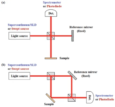
This motivates us to devise a way to use the components we have used for FF-OCT in an FD-OCT configuration. FD-OCT can be implemented either with swept-sources (SS-OCT) or by using spectrometers such as spectral-domain OCT (SD-OCT).
Experimental method .1 General setup
This is because we align the camera to have the spectrum centered around the known center wavelength of the source. With these settings, use a single surface reflector as a sample in the FD-OCT device.
Data processing
Improved signal-to-noise ratio in spectral domain compared to optical coherence tomography in time domain. High resolution corneal and single pulse imaging with line field spectral domain optical coherence tomography.
Instrumentation 1 System architecture
System design considerations regarding axial point-spread-function and depth range
Interference is only observed when the optical path difference (OPD) between the reference and the sample is within the coherence length of the source. For example, the chromatic aberration of the objective lens would change the local effective bandwidth and degrade the axial PSF [13].
Lateral scanning approaches
This axial displacement sensitivity was empirically shown to be often better than one per thousand of the FWHM of the axial PSF. As has been shown, both the width of the axial PSF and the image depth range are proportional to the square of the center wavelength of the source λ02.
Calibration
- Spectral nonlinearity calibration
- Depth scale calibration
- Field flatness audit
- Lateral scanning field audit and calibration
For example, field curvature can be caused by incorrect positioning of x and y scanning mirrors displaced from the pupil plane of the objective lens. The objective size covers the entire lateral field of view (FOV) of the OCT system.
Methodology for film thickness and refractive index metrology with OCT
Simultaneous film thickness and refractive index metrology by evaluating optical distortion induced by a film sample in the sample path
From the metrics evaluated from a dot grid target, calibration can be applied to correct the non-orthogonality of the two scan axes or calibrate the distortion of the field. From the metrics evaluated from a dot grid target, calibration can be applied to correct the non-orthogonality of the two scan axes or calibrate the distortion of the field.
![Figure 5a shows an example of a raw gray-scale x-y plane image of a dot grid target acquired by an SS-OCT system with 2-D x-y stages for lateral scanning [19].](https://thumb-ap.123doks.com/thumbv2/1libvncom/9201738.0/106.765.115.655.80.387/figure-shows-example-target-acquired-stages-lateral-scanning.webp)
Simultaneous film thickness and refractive index metrology by hybrid confocal-scan FD-OCT
Examples
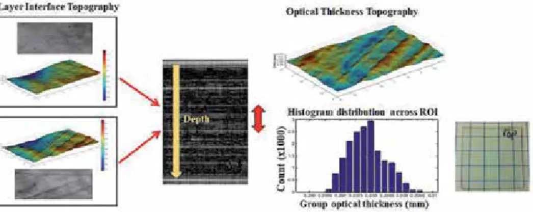
Film interface and thickness topography
The source's instantaneous linewidth is approximately 0.2 nm, resulting in an image depth range of approximately 1 mm. Based on the acquired OCT imaging data, a surface segmentation algorithm is applied to produce a 3D visualization of the surface profiles of interfaces between the layers.
Metrology of film thickness through depth
Two sets of 3D-OCT data covering the upper and lower parts of the sample were collected and volumetrically plotted as shown in Figure 10. Nondestructive metrology of the layer thickness profiles across the depth of a multilayer monolithic polymer sample.
Simultaneous refractive index and thickness metrology
A cross-sectional image of the bottom 11 layers of the sample after being cut and imaged under a light microscope. i) Quantitative comparison of the layer thickness profiles of the lower 11 layers obtained from OCT and microscope measurements (adapted from [31]). It is also shown in Figure 11a that the measured cumulative thickness increases more rapidly near both surfaces of the sample.
Summary and perspectives
Volumetric representation and metrology of spherical gradient refractive index lenses imaged by angle-scanning optical coherence tomography system. Refractive index and thickness characterization of biological tissues using combined multiphoton microscopy and optical coherence tomography.
Water scarcity
Membrane technology
The most widespread classification is based on the pore size of the membrane, while the removal of unwanted contaminants is related to the pore size of the membrane. Another classification is based on the geometry of the membrane used in the process (i.e. flat plate, spiral wound, tubular and hollow fiber).
Membrane fouling
The development of membrane fouling on the membrane surface is considered a bottleneck of membrane filtration processes. Particle fouling is the result of the accumulation of suspended particles of different nature on the membrane surface.
Fouling characterization
In-situ nondestructive fouling characterization
The structural analysis of the fouling layer deposited on a membrane coupon consists of the use of imaging techniques. The main limitation of the conventional imaging techniques in the characterization of the growth is represented by the impossibility of collecting data over time.
Biofilm characterization with OCT
- Morphology analysis
- Monitoring the fouling growth under continuous operation
- OCT monitoring in spacer-filled channel
- Monitoring inorganic fouling
- Using the OCT to improve fluid dynamic simulation
Indeed, the main objective of fouling characterization is to understand the impact of deposited biomass on system performance [10]. One of the main objectives of structural fouling analysis is to evaluate the impact of biomass deposited on the membrane on performance.
Drying process of colloidal droplets
In the next stage, the formation of the nematic phase (N) shifted the isotropic (I)-nematic phase boundary to the center. In the case of the water-ethanol droplet with the preferential evaporation of ethanol, the binary liquid near the air-water interface was denser than the bulk.
Drying process of colloidal latex droplets
In the experiment, a droplet containing sunset yellow FCF (SSY), a dye belonging to the LCLC family, was placed on a premium coverslip of the substrate. In the horizontal direction, the evaporation rate is faster at the edge of the drop than in the center.
Drying process of latex coats
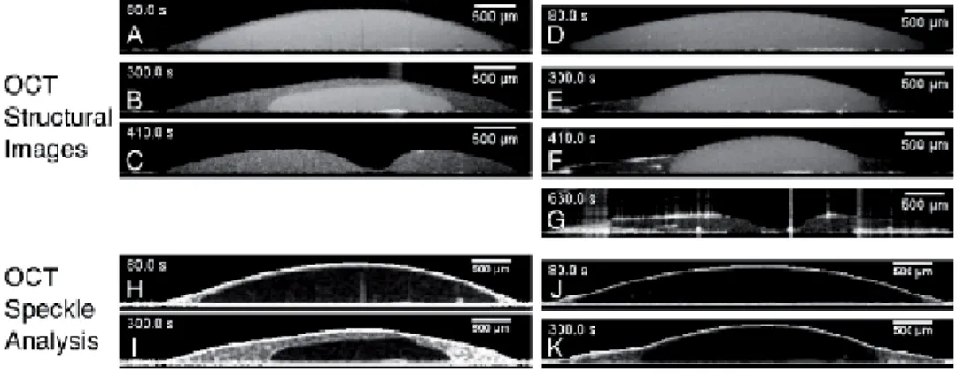
The combination of OCT with gravimetric and video measurements can fully characterize the drying process of polystyrene latex coating [30]. In the final drying phase, the latex coating remains uniform without significant changes in the intensity or thickness of the coating.
Discussions
Formation of shear bands is observed in the polystyrene latex coat, shown in 2D OCT structural image in Figure 4D. At ~212 min, the shear band structure begins to form, indicated by the bright crosses within the latex. The shear band is assumed to be attributed to the disruption of packed latex particles due to the internal.
Conclusions and future perspectives
OCT can provide cross-sectional images to observe the internal structures of the colloidal droplets and latex coatings. For latex coatings, the field of view (FOV) of a standard OCT system (a few millimeters square) only covers a small area of the latex coating.
An overview of recent applications of OCT in heritage science
The capabilities of combining OCT and nonlinear microscopy (NLM) were investigated by Liang et al. As a result, the results were used to plan a restoration campaign (which has already been completed).
OCT instrument designed for heritage science 1 Opto-mechanical details
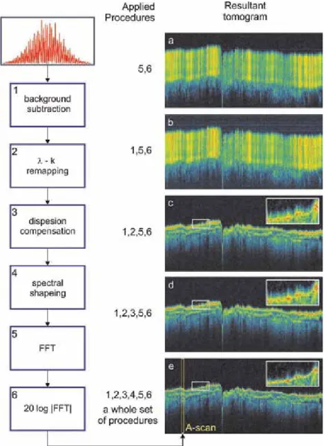
Data processing and software
Assuming the earlier preparation of the necessary data common to all spectra (in particular, the vectors used in the procedures of numerical dispersion compensation and λ-k remapping [42]), this analysis does not require complex calculations: BG subtraction requires the calculation of the difference of two vectors (2048 elements each) ;. The influence of individual numerical procedures on the quality of the OCT tomogram used in an individual A-scan.
Examples of structural images of artwork
They are displayed (like all tomograms in this chapter) with false color scale: structures that strongly reflect/scatter the probing light. Through glass OCT examination of the miniature from the collection of the National Museum in Cracow (MNK III-min cm2, reverse paintings on glass.
Application for varnish removal assessment
In this case it is the surface of the opaque paint layer, clearly visible on the tomograms. Therefore, the second tomogram had to be shifted in both directions to achieve the desired paint film correlation (Fig. 4b).
Conclusions
Using optical coherence tomography to reveal the hidden history of the "Virgin Lansdowne of the. Application of optical coherence tomography (OCT) for real-time monitoring of paint layer consolidation on Hinterglasmalerei objects.
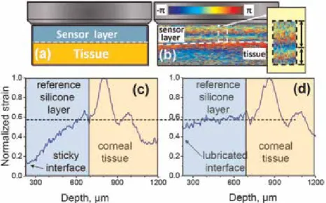
Basic principles used in OCE
The idea of using quasi-static uniaxial stress to estimate Young's modulus was proposed for ultrasound [7] and was transferred to OCT in [6]. It can be shown that the phase of the OCT signal can be more tolerant to strain-induced decorrelation [21].
Local estimates of strains in phase-sensitive OCE using the “vector method”
Schematic evaluation of the axial phase gradient in the vector approach for laterally nearly homogeneous strains. Schematic evaluation of the axial phase gradient in the vector approach adapted to laterally inhomogeneous strains with non-horizontal phase variation isolines.
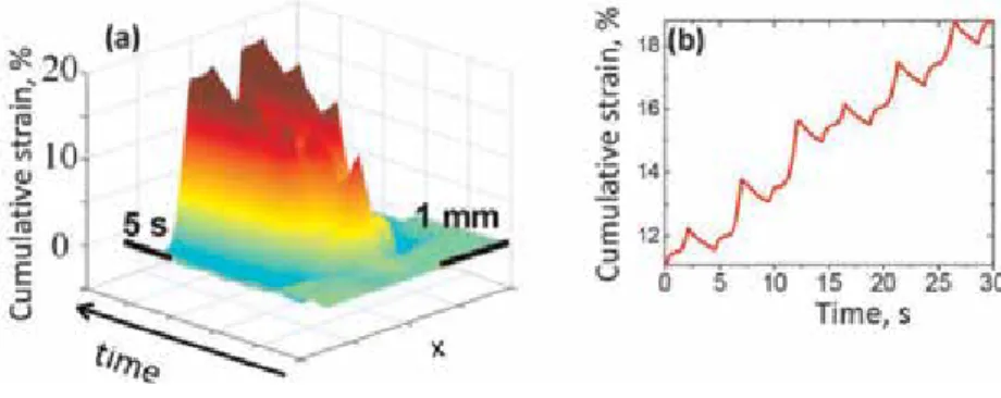
Examples of the vector method application for strain mapping by elastographic processing real OCT scans
Examples of the vector method application for strain mapping by elastographic processing of real OCT scans by elastographic processing of real OCT scans. It can be said that the choice of the method of strain accumulation depends on the specific problem.
Obtaining of quantitative stress-strain curves and estimation of Young modulus in phase-sensitive compressional OCE
Now consider the possibilities of the developed strain mapping approach for quantitative mapping of Young's modulus in the studied samples. Consequently, the response to such compression is determined by the Young's modulus of the material.
Spectral-domain OCT with a visible broadband light source
The axial resolution of an OCT image is controlled by the central wavelength (λ0) and bandwidth (Δλ) of the low-coherence light source. Figure 1(b) shows a spectrum of the light source reflecting from the reference mirror detected with the spectrometer.
Surface-structure observations and measurements of RWGs and periodic patterns with Vis-OCT
Sample preparations
Height and width measurements of isolated RWGs
The peak intensity at the surface of the substrate was smaller (approx. -5 dB) than that at the surface of the RWG. As seen in Figure 4(b), the reflection peaks at the surfaces of the substrate and the RWG can be clearly distinguished.
Soft mold for NIL
The surface line of the substrate and the RWG indicated by a red dotted line in each OCT image were determined at the reflection peak position. Figure 6(a), (b) shows the comparison of the measured heights and widths of different RWGs between vis-OCT and SEM.
Profile imaging of semitransparent thin films
Sample of stacked thin layers
The refractive index of the Al0.3Ga0.7As layer varies in the range of 3.5–4.8 as a function of the wavelength of broadband visible light, as shown in the upper part of Figure 9(a). In addition, the Al0.3Ga0.7As layer exhibits optical absorption depending on the wavelength due to the bandgap energy.
Numerical simulations
Figure 9(b) shows simulated spectra of the broadband visible light source transmitted through an Al0.3Ga0.7As layer with different thicknesses in the range of 250-2000 nm. This indicates variations of the transmitted spectral shape of the visible broadband light with the thickness of the Al0.3Ga0.7As layer, resulting in the variation of nAlGaAs with the spectral changes.
Profile measurements and imaging with the Vis-OCT
The physical thickness of the photoresist film can therefore be estimated from the optical thickness divided by e.g. The physical thickness of the AlGaAs layer was set to 512 nm in. a) 2D model for the FDTD simulation.
Conclusions
In addition, the broadband visible light spectrum used in the FDTD simulation had an ideal Gaussian shape (symmetric at the central wavelength), which differs from the actual spectrum of the light source used in fish OCT. Furthermore, we obtained a 2D profile image of the sample by collecting profiles in the lateral direction, as shown in Figure 12.