This is based on feedback from teachers, students, and my occasional re-reading of the book. Yakovenko of the University of Maryland for spotting many errors in the first printing and going out of his way to point them out to me.
Prelude
In the rest of the book, the postulates are invoked to formulate and solve a variety of quantum mechanical problems. The answer to each exercise is given <~either together with the exercise or at the end of the book.
Contents
Mathematical Introduction
Linear Vector Spaces: Basics
Consider the set of all entities of the form (a, b, c) where the entries are real numbers. Expansion coefficients V; of a vector in terms of an independent linear basis (I i)) are called the components of the vector in that basis.
Inner Product Spaces
We are now ready to get a concrete formula for the inner product in terms of the components. The inner product (VI W) is given by the matrix product of the transpose conjugate of the column vector representing I V) with the column vector representing I W:.
Dual Spaces and the Dirac Notation
- Expansion of Vectors in an Orthonormal Basis
However, there is nothing wrong with the first point of view of associating a scalar product with a pair of columns or kets (not referring to another double space) and living with the asymmetry between the first and second vectors in the inner product (which one to transpose conjugate ?). Subtract from the second vector its projection along the first, leaving only the part perpendicular to the first.
- Subspaces
In terms of the objects I i)(il, which are linear operators and which by definition act on IV) to give li)(il V), we can write the above as. Thus, the matrix representing the product of operators is the product of the matrices representing the factors.
- Functions of Operators and Related Concepts
- Generalization to Infinite Dimensions
Now we have only one equation, instead of the two (n-1) we are used to. Note that, in view of degeneracy, I W;) no longer refers to a single ket, but to a generic element in the eigenspace w::;;. Using the results on the trace and the determinant from the last problem, show that the eigenvalues of the matrix .
Because of the complete symmetry of the sphere, it is clear that each direction is its own direction of rotation. As a first step, we rewrite Eq. where the elements of the Hermitian matrix Qii are. The basis II), 12) is very desirable physically, for the components of jx) in this basis (x1 and x2) have the simple interpretation as displacements of the masses.
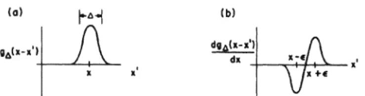
If we now take Jet n to infinity, we get, according to the usual definition of the integral, . Note that this is only defined in the context of an integration: the integral of the delta function o(x- x') with any smooth functionf(x') isf(x). As in the case of the K operator, one usually suppresses the integral over the common index since it is made trivial by the delta function.
Review of Classical Mechanics
The Two-Body Problem
Since the particles interact with each other and nothing external, it follows that the potential between them depends only on the relative coordinate r = rt - r2 and not on the individual positions r1 and r2. The corresponding conserved momentum is, of course, the three components of the total momentum, which are conserved in the absence of external forces. The main features of Eq. l) The problem of two interacting particles has been transformed into that of two fictitious particles that do not interact.
One clear way to do this is to go to the CM frame in which i"cM = 0, so that CM is completely eliminated in the Lagrangian. If we choose, we can easily return to the r1 and r2 coordinates at the end, using Eq.
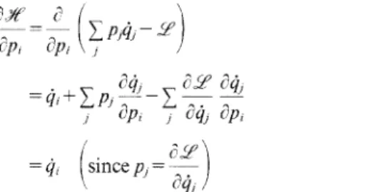
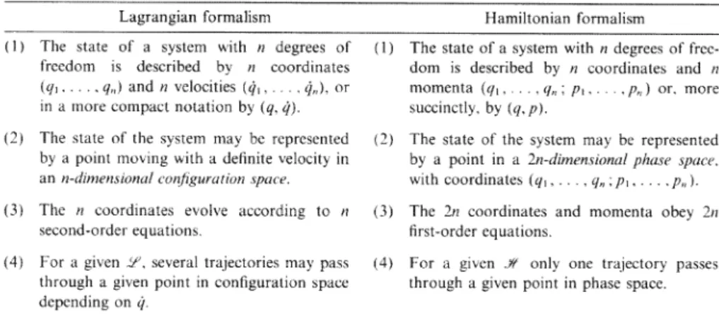
In the Hamiltonian formalism, the roles of q and p are exchanged: the Lagrangian .!l'(q, q)t is replaced by a Hamiltonian Jf(q,p), which generates the equations of motion, and q becomes a derived quantity, . 2.5.6) that all the x;s to be eliminated have been rewritten as functions of the allowed variables in g. The passage from .f[e·m to its Legendre transform .Xt'em is not sensitive in any way in the face of the speed-dependent nature of the force.
If the correct force laws are generated, ,/{,., will do the same, since the dynamic content of the schemas is identical. In contrast, the speed-independence of the force was assumed to show that the numerical value of ,Y{ is T + V, the total energy. The answer, of course, is that .yf is more than just T + q¢; it is T + qr/J written in terms of the appropriate variables, specifically in terms of p and not v.
Cyclic coordinates, Poisson brackets and canonical transformations Cyclic coordinates are defined here as in the Lagrangian case and have the.
Cyclic Coordinates, Poisson Brackets, and Canonical Transformations Cyclic coordinates are defined here just as in the Lagrangian case and have the
Now there is something very disturbing about Eq. 2.6.1): the vector potential A appears to have dropped out along the way. This is as it should be, for we expect the momenta's response to a coordinate transformation (eg a rotation) to be a purely kinematic matter. Thus the numerical value of the Lagrangian is unchanged under (q, q)-+ (ij, lj); for (q, q) and (ij, lj) refer to the same physical state.
Given one set, (q,p), we can obtain another, (ij,p), by the point transformation, which is a special case of the canonical transformation. We would like to draw here the equation. 2.7.9), which gives the moment transformation under a coordinate transformation in the configuration space:. Use the chain rule and the fact that q=q(q) and not q(q, q) to derive Eq. 4) Verify by calculating BP in Eq.
Now consider a limited class of transformations, called regular transformations, which preserve the range of the variables: (q,p) and (ij,p) have the same.
Symmetries and Their Consequences
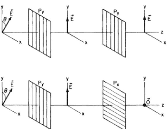
Consider a two-particle system whose Hamiltonian is invariant under the translation of the entire system, i.e. both particles. Convince yourself that the states of the two particles at later times are not associated with the same transformation. In the case of sound waves, tp is the excess air pressure above normal, while in the case of electromagnetic waves, tp can be any component of the electric field vector E. The analogs of q and q for a wave are tp and 1jr at each point r, provided that tp obeys a second-order wave equation in time, which e.g. a) When a wave w=e''c.-wn is incident on the screen with either slit S1.
However, time averages of energy and momentum flow are still proportional to intensity (as defined above) in the case of plane waves.]. However, these subtleties can wait.] The entire experiment can be understood in terms of this hypothesis as follows. For any reasonable value of parameters a and d (see Figure 3.1 b), the interference pattern would be so dense in x that our instruments will measure only the smooth average, which will obey.
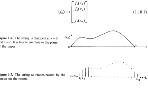
The dynamics of the particle is then the dynamics of this function '!f(X, t) or, if we think of functions as vectors in an infinite dimensional space, of ket I lfl{t).
The Postulates-a General Discussion
The Postulatest
Discussion of Postulates 1-111
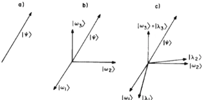
Then. which is the modulus of the square of the projection I 'If) in the degenerate eigenspace. This is part of the information contained in the lf!(x) = (x llf!), llf!) components in the base X. However, this information is nothing compared to the complete specifications of the state immediately after the measurement.).
But we cannot repeat the experiment with this particle, because after the measurement the state of the particle is I A1). In the non-degenerate case, this also implies the invariance of the state vector. Compatibility therefore generally implies the invariance under the second measurement of the eigenvalue measured in the first.
A convenient way to put all this information together is in the form of the density matrix (which is actually an operator that somehow becomes a matrix).
A complicated procedure exists for quantization in non-Cartesian coordinates, but we won't discuss it, since the recipe eventually reproduces what the Cartesian recipe (which seems to work) gives so easily. Apart from a brief discussion of these towards the end of the program, we will not address these issues. On such a basis, the vectors would appear frozen, but the operators, which were constant matrices in the fixed basis, would now appear to be time dependent.
In the course of our study, we will encounter a time-dependent problem involving spin that can be solved exactly. We will also study a systematic approximation scheme for solving problems with .. where H0 is a large time-independent piece and H1{t) is a small time-dependent piece. Since V(X) is usually a more complicated function of X than T is of P, one prefers the X basis. H]E)=EiE) becomes the second-order equation in the X basis.
For pedagogical reasons, we will limit ourselves in the next few chapters to problems of a single particle in one dimension.
Simple Problems in One Dimension
The Free Particle
In terms of the ideas discussed in the past, we are using the eigenvalue of a compatible variable P as an additional label within the degenerate space with respect to the energy. In the absence of anything defining an absolute time in the problem, only the time changes have physical significance.] Whenever we set t' = 0, we will revert to our old convention and write U(x, t; x', 0) as simply U(x, t; x'). There is an unwritten law that states that the derivation of the free particle propagator follows from its application to the Gaussian bundle.
This is just one of the consequences of Ehrenfest's theorem, which states that classical equations respected by dynamical variables will have counterparts in quantum mechanics as relations between expectation values. The increasing uncertainty in position is a reflection of the fact that any uncertainty in the initial velocity (ie momentum) will be reflected over time as an increasing uncertainty in position. Although we are able to understand the propagation of the wave packet in classical tennets, the fact that the initial propagation !\ V(O) is inevitable (given that we wish to specify the position to an accuracy A) is a purely mechanical property quantum. .
This and similar questions will be dealt with in more detail in the next chapter.
The Particle in a Box
Show that the probability of finding a particle in the ground state of the new box Hint: Expand I ty) in its own basis H.). But charge is also conserved locally, a fact that is usually expressed in the form of a continuity equation. This result is obtained by expressing and the variance of the norm in the coordinate base: so.
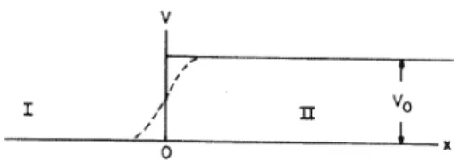
A schematic description of the wave function long before and long after it hits the step. We follow the standard procedure to find the fate of the incident wave packet, lf/1. When we come to dispersion in three dimensions, we will assume that the equivalence between the two approaches holds.
Let's label the I and II regions on the left and right of the screen.