This rewriting of the integral is based on a selection of integration points, i D n which are distributed on the interval Œa; b. Starting from (3.5), the different integration methods will differ in the way they approach each integral on the right-hand side. In particular, we want to use an integral that we can calculate by hand so that the accuracy of the approximation methods can be easily assessed.
We can therefore calculate the exact value of the integral as V .1/V .0/1:718 (rounded to 3 decimal places for convenience). Strictly speaking, for example, writing “the trapezoidal method” should imply the use of only one trapezoid, while “the compound trapezoidal method” is the most correct name when multiple trapezoids are used. Now we calculate our special problem by calling application() as the only statement in the main program.
How much do we need to change in the previous code to calculate the new integral?
The Composite Midpoint Method
The General Formula
Implementation
Comparing the Trapezoidal and the Midpoint Methods The next example shows how easy we can combine the trapezoidal and
The trapezoidal and midpoint methods are just two examples in a jungle of numerical integration rules. Different methods differ in the way they construct evaluation scores and weights.
Testing
- Problems with Brief Testing Procedures
- Proper Test Procedures
- Finite Precision of Floating-Point Numbers
- Constructing Unit Tests and Writing Test Functions
Of course it is completely impossible to say whether 0.1 is the correct error value. Fortunately, the increment shows that the error stays around 0.3 in the program with the error, so the procedure of testing with the increment and checking that the error decreases indicates a problem in the code. That is, the error should be reduced to correct code faster than to error code.
The unit test should be independent in the sense that it can be run without the results of other tests. A strong test when we can calculate exact errors is to see how quickly the error goes to zero asnrows. In the trapezoid and midpoint rules, it is known that the error depends on n as n2 as n.
We can therefore choose a linear function and construct a test function that checks equality between the exact analytical expression of the integral and the number calculated by the implementation of the trapezoidal method. The idea of a corresponding unit test is then to run the algorithm for some values, calculate the error (the absolute value of the difference between the exact analytical result and that produced by the numerical method) and check that the error has an approximately correct asymptotic behavior. , i.e. that the error is proportional to ton2 in the case of the trapezoidal and midpoint method. Suppose we have a calculationa + band we want to check that the result is what we expect.
We see that all numbers have an imprecise digit on the 17th decimal place. When we calculate with real numbers, those numbers appear imprecise on the computer, and arithmetic operations with imprecise numbers lead to small rounding errors in the final results. As we show below, these tolerances depend on the size of the numbers in the calculations.
Solving the problem without numerical errors We know that the trapezoidal rule is exact for linear integrands. Proving the correct rates of convergence In this case by integration, it is known that the approximation errors in the trapezoidal rule are proportional ton2, which is the number of subintervals used in the composite rule.
Vectorization
Measuring Computational Speed
Double and Triple Integrals
The Midpoint Rule for a Double Integral
Integrals in the x direction use hx and nxforhandn, andias counter. a g.x/dx, which can be approximated by the midpoint method:. Direct derivation The formula (3.25) can also be derived directly in the two-dimensional case by applying the idea of the midpoint method. The idea of the midpoint method is to approximate a constant for each cell, and evaluate the constant at the midpoint.
ŒaCihx; aC.iC1/hxŒcCj hy; cC.jCl/hy; and the midpoint is.xi; yy/with. Reusing code for one-dimensional integrals It is very natural to write a two-dimensional midpoint method, as we did in functionmidpoint_double1, when we have the formula (3.25). But we could alternatively ask, just as we did in mathematics, whether we can reuse a well-tested implementation for one-dimensional integrals to compute double integrals.
The answer is yes, if we think like in mathematics: calculate the double integral as the middle rule for integratingg.x/and define g.xi/ in terms of the middle rule over f in their coordination. An important advantage of this implementation is that we reuse the well-tested function for the standard one-dimensional center rule and that we use the one-dimensional rule exactly as in mathematics. The rule of the middle is exact for linear functions, no matter how many subintervals we use.
Since a test function should not have a print statement, we simply comment it out as we did in the function listed above. The derivation of a formula for the double integral and the implementations follow exactly the same ideas as we explained with the midpoint method, but there are more terms to write in the formulas. That exercise is a very good test of your understanding of the mathematical and programming ideas in the current section.
The Midpoint Rule for a Triple Integral
However, it's somewhat annoying to have a function that's completely silent when it works - are we sure all things are calculated correctly? It is therefore strongly recommended to include a print statement during development so that we can monitor the calculations and be confident that the test function does what we want. This exercise is a very good test of your understanding of the math and programming ideas in this section. and you want to approximate the integral with a midpoint rule.
Following the ideas for the double integral, we split this integral into one-dimensional integrals:. Note that we can apply the ideas under Direct derivation at the end of Section.3.7.1 to arrive directly at (3.26): divide the domain intonxnynzcells of volumes hxhyhz; approximated by a constant, evaluated at the center.xi; yy; zk/, in each cell; and sum the cell integralshxhyhzg.xi; yy; zk/. Implementation We follow the ideas for implementing the midpoint rule for a double integral.
Monte Carlo Integration for Complex-Shaped Domains Repeated use of one-dimensional integration rules to handle double and triple inte-
The integral can be evaluated using this Monte Carlo integration method:. embed geometry˝in a rectangular areaR 2. draw a large number of random points.x; y/inR 3. count the fraction of q points that are inside˝. evaluate the average off,fN, at points within˝ 6. evaluate the integral as A.˝/fN. Note that A.R/ is trivial to calculate because R is a rectangle while A.˝/ is unknown. However, if we assume that the proportion of A.R/ occupied by A.˝/ is equal to the proportion of random points inside˝, we obtain a simple estimate for A.˝/. To get an idea of the method, consider a circular domain embedded in a rectangle as shown below. A collection of random points is illustrated by black dots. f .x; y/dxdy can be written like this:. n^2 is the number of random points.
The correct answer is 3, but Monte Carlo integration is, unfortunately, never exact, so it is impossible to predict the outcome of the algorithm. All we know is that the evaluated integral must approach 3 as the number of random points goes to infinity. Also, for a fixed number of points, we can run the algorithm multiple times and get different numbers that fluctuate around the exact value, since different sample points are used in different calls to the Monte Carlo integration algorithm.
It is known mathematically that the standard deviation of the Monte Carlo estimate of an integral converges asn1=2, which is the number of samples. Test function for function with random numbers To make a test function, we need a unit test that has identical behavior every time we run the test. This seems difficult when random numbers are involved, because these numbers are different every time we run the algorithm, and thus each run produces a (slightly) different result.
Provided that the test function always uses this seed, we should get exactly this result every time the MonteCarlo_doublefunction is called. As in the test case above, we experience better results with a larger number of points. When we have such evidence for a working implementation, we can turn the test into a proper test function.
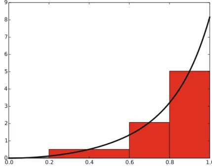
Hand calculations for the trapezoidal method
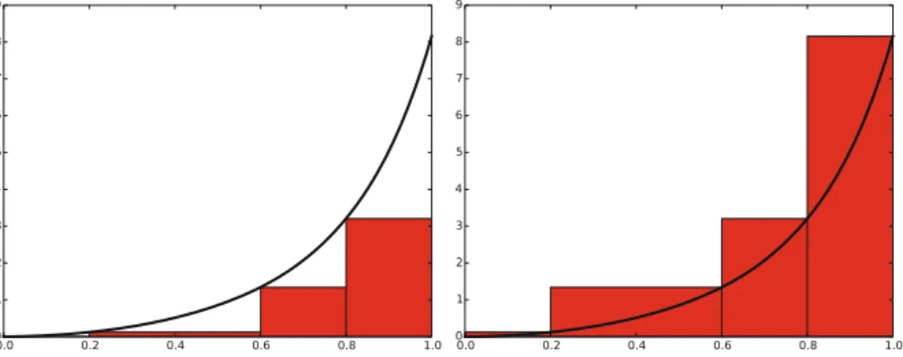
Hand calculations for the midpoint method
Hand-calculations with sine integrals We consider integrating the sine function: R b
Make test functions for the midpoint method
Explore rounding errors with large numbers
Rectangle methods
To answer this question, we can introduce an iterative procedure where we compare the results produced by thorns2n intervals, and if the difference is less than 2, the value corresponding to 2 is returned. Tip It might be a good idea to organize your code so that the function adaptive_..integration can be easily used in future programs you write. a) Write a function. Remarks The type of method explored in this exercise is called adaptive because it attempts to adjust the value to meet a particular error criterion.
The true error can very rarely be calculated (since we don't know the exact answer to the calculation problem), so one has to find other indicators of the error, such as this one where the changes in integral value as the number of intervals doubles are taken to reflect the error.
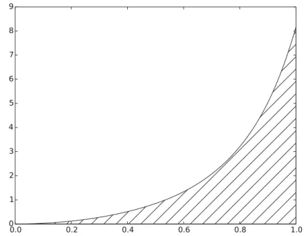
Integrating x raised to x Consider the integral
Let's say we want to use the trapezoidal or median method to calculate the integral Rb. a f .x/dx with an error smaller than the prescribed tolerance. Integrandxx does not have an antiderivative that can be expressed by standard functions (visit http://wolframalpha.com and type integral(x**x,x) to verify that our claim is correct. Note that Wolfram alpha provides you answer, but this answer is an approximation, not exact.
This is because Wolfram alpha also uses numerical methods to arrive at the answer, just as you will in this exercise).
Integrate products of sine functions In this exercise we shall integrate
Revisit fit of sines to a function
A remarkable property of the trapezoidal rule is that it is exact for integralR sinnt dt (when subintervals are of equal size). Use this property to create a function test_integrate_coeff to verify the implementation of integrate_coeffs. e) Implement the choicef .t / D 1t as a Python function f(t) and call integrate_coeffs(f, 3, 100) to see what the optimal choice of b1 is; b2; b3is. f) Make a function plot_approx(f, N, M, filename) where you plotf(t) together with the best approximationSN calculated as above, using M intervals for numerical integration.
Derive the trapezoidal rule for a double integral